Chapter 22 Visualizing phylogenetic networks
We will be working with both the DensiTree application from BEAST and the phangorn package in R.
22.1 Using DensiTree
When you ran your Bayesian analysis, you created a distribution of trees. You summarized this distribution when you looked at the posterior estimates of support for the nodes and clades, but there is a lot more information we can get from this distribution.
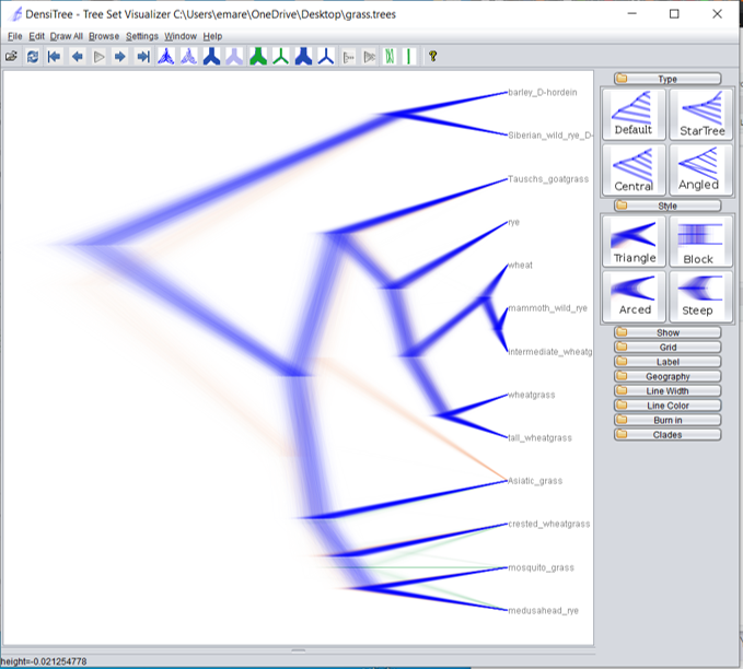
Open DensiTree on your personal computer. (DensiTree should have been installed when you downloaded BEAST.) Click on File, then Load and choose your .trees file that was created when you ran BEAST. All the trees in the distribution will be drawn in a fuzzy-looking tree. The darker the line, the more consensus there is among your tree distribution that the branch exists.
In the grass example, we see branches in three separate colors - blue, orange, and green. (I changed the default colors by clicking on “Line Color” in the menu on the right side of the screen. If you open it and then open the “Line Colors” option, you can change your colors as well.) The blue branches are branches supported by the majority of the tree distribution, while the orange and green branches represent alternate branching patterns.

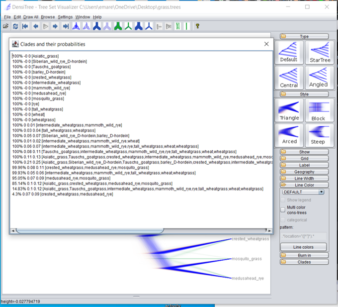
The orange and green colors are very light because those alternate branching patterns show up in only a small percentage of the tree distribution. We can see the percentage if we click on “Help” and then “View Clades.”

There’s not much disagreement among the trees in the posterior distribution for our grass example. The main disagreement is with the placement of the Asiatic grass sample; 85% of the trees place Asiatic grass with the crested wheatgrass/medusahead rye/mosquito grass clade, which 15% place it in a different position.
I have been using the words “probability” and “percentage” interchangeably when talking about the Bayesian posterior tree distribution. Although probability and percentage aren’t usually the same thing, in this case they are. We are estimating the probability of topologies by calculating the percentage of the tree distribution with the desired topology.
22.2 Networks in R
phangorn offers an algorithm called consensusNet to visualize conflicting topological relationships from our data. This algorithm builds networks similar to the Huson example above using previously-generated analyses files.
We have two options for our input. consensusNet takes a list of trees as the input (which R sees an an object of class multiPhylo), so we can either load the bootstrap trees from the ML analysis or the posterior distribution of trees from the Bayesian analysis. Here we will do both with the grass dataset so we can compare the networks. (Notice that we need to use two different commands to load the trees into R - the two tree files are saved in two separate formats. The ML trees are saved in Newick format, while the Bayesian trees are saved in Nexus format.)
library(phangorn)

grass.ml <- read.tree("grass_ml_bootstrap.tre")
grass.bayes <- read.nexus("grass_bayes.trees")
After we load our trees, we run the consensusNet command. This command takes two arguments. The first is the tree file, while the second is the bootstrap value threshold. For this example, we’ll set the threshold at 0.1, meaning we will see all the possible nodes with at least a bootstrap support or posterior density of 0.1.
cnet.ml <- consensusNet(grass.ml, .1)
cnet.bayes <- consensusNet(grass.bayes, .1)

plot(cnet.ml, show.edge.label=TRUE)
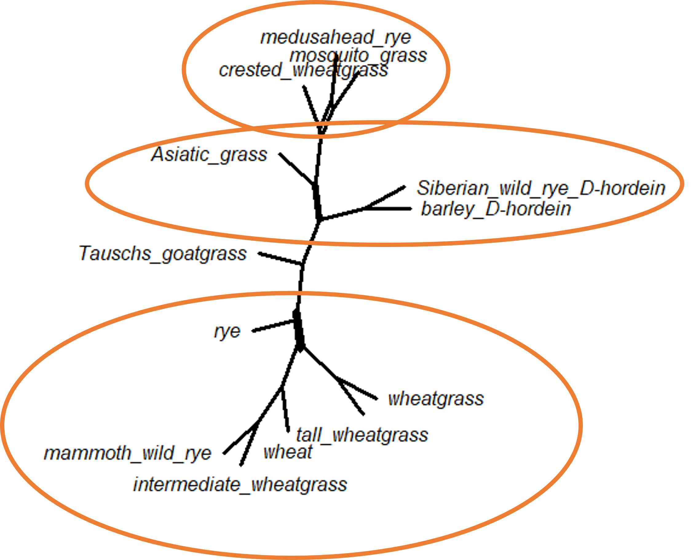
We can see there are very few alternate topologies in the bootstrap trees (which we already knew would be the case, given the high bootstrap support in the original ML tree!), but there are a couple of splits. The first suggests that crested wheatgrass is sometimes in a polytomy with medusahead rye and mosquito grass, instead of splitting from that clade earlier. The second split suggests that some trees has Asiatic grass splitting from the main tree as the basal node and sometimes clusters with the crested wheatgrass/medusahead rye/mosquito grass clade. Finally, the last split changes the position of rye.

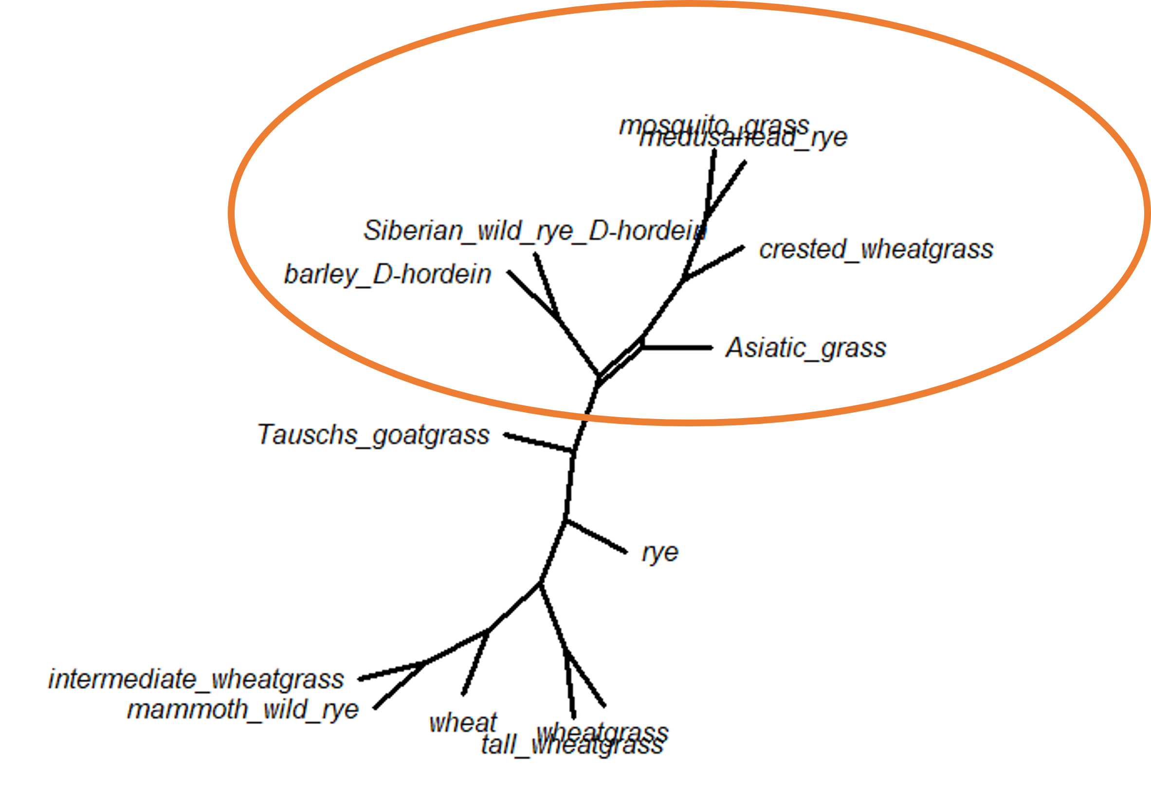
There is only one split in the Bayesian network - the placement of Asiatic grass taxon. We have seen this already in the DensiTree diagram, but it does look a bit different in network form. This particular split shows up in both the ML bootstrap network and the Bayesian posterior distribution network.
We can also add the support values for each split (the bootstrap values for the ML network, or the posterior probabilities for the Bayesian network) by changing the show.edge.label command to equal TRUE. Be careful, though, as this can make the network very difficult to read.
## R version 4.3.2 (2023-10-31)
## Platform: x86_64-pc-linux-gnu (64-bit)
## Running under: Ubuntu 22.04.4 LTS
##
## Matrix products: default
## BLAS:   /usr/lib/x86_64-linux-gnu/openblas-pthread/libblas.so.3
## LAPACK: /usr/lib/x86_64-linux-gnu/openblas-pthread/libopenblasp-r0.3.20.so;  LAPACK version 3.10.0
##
## locale:
##  [1] LC_CTYPE=en_US.UTF-8       LC_NUMERIC=C
##  [3] LC_TIME=en_US.UTF-8        LC_COLLATE=en_US.UTF-8
##  [5] LC_MONETARY=en_US.UTF-8    LC_MESSAGES=en_US.UTF-8
##  [7] LC_PAPER=en_US.UTF-8       LC_NAME=C
##  [9] LC_ADDRESS=C               LC_TELEPHONE=C
## [11] LC_MEASUREMENT=en_US.UTF-8 LC_IDENTIFICATION=C
##
## time zone: Etc/UTC
## tzcode source: system (glibc)
##
## attached base packages:
## [1] stats     graphics  grDevices utils     datasets  methods   base
##
## other attached packages:
## [1] phangorn_2.11.1 ape_5.7-1
##
## loaded via a namespace (and not attached):
##  [1] sass_0.4.8       utf8_1.2.4       generics_0.1.3   xml2_1.3.6
##  [5] lattice_0.21-9   stringi_1.8.3    hms_1.1.3        digest_0.6.34
##  [9] magrittr_2.0.3   grid_4.3.2       evaluate_0.23    timechange_0.3.0
## [13] bookdown_0.41    fastmap_1.1.1    Matrix_1.6-1.1   rprojroot_2.0.4
## [17] jsonlite_1.8.8   processx_3.8.3   chromote_0.3.1   ps_1.7.6
## [21] promises_1.2.1   httr_1.4.7       fansi_1.0.6      ottrpal_1.3.0
## [25] codetools_0.2-19 jquerylib_0.1.4  cli_3.6.2        rlang_1.1.4
## [29] cachem_1.0.8     yaml_2.3.8       parallel_4.3.2   tools_4.3.2
## [33] tzdb_0.4.0       dplyr_1.1.4      fastmatch_1.1-4  vctrs_0.6.5
## [37] R6_2.5.1         lifecycle_1.0.4  lubridate_1.9.3  snakecase_0.11.1
## [41] stringr_1.5.1    janitor_2.2.0    pkgconfig_2.0.3  pillar_1.9.0
## [45] bslib_0.6.1      later_1.3.2      glue_1.7.0       Rcpp_1.0.12
## [49] xfun_0.48        tibble_3.2.1     tidyselect_1.2.0 knitr_1.48
## [53] igraph_2.0.2     nlme_3.1-164     htmltools_0.5.7  websocket_1.4.2
## [57] rmarkdown_2.25   webshot2_0.1.1   readr_2.1.5      compiler_4.3.2
## [61] quadprog_1.5-8   askpass_1.2.0    openssl_2.1.1