
Chapter 18 Estimating a tree using Maximum Likelihood
We will be using the phangorn package in R to estimate maximum likelihood methods.
phangorn has three possible tree permutation methods available in its maximum likelihood commands. The first is the nearest neighbor interchange (NNI) method, which we used in our parsimony estimation. However, the NNI algorithm can sometimes get stuck on a local optimum in tree space (especially as the tree gets larger). The other two (the stochastic approach and the likelihood ratchet) will make random NNI rearrangements to the tree, which can allow the tree to escape local optima and instead find a global optimum of our tree-searching space.
18.1 Creating a starting tree
phangorn requires a starting tree for maximum likelihood searches. The tree itself doesn’t matter much, but generally people supply a neighbor joining tree because they can be generated quickly.
library(phangorn)

grass.align <- read.phyDat("grass_aligned-renamed.fasta", format = "fasta")

dist <- dist.ml(grass.align)
nj.tree <- nj(dist)
You can also upload your previously-generated neighbor joining tree and use that instead of creating a new one (just make sure that you used the same sample names in both your renamed fasta file and your neighbor joining tree).
18.2 Calculating likelihood score
Once you have both a tree and your fasta file loaded, you can calculated a likelihood score using the pml command.
## model: JC
## loglikelihood: -12533.76
## unconstrained loglikelihood: -20944.97
##
## Rate matrix:
##   a c g t
## a 0 1 1 1
## c 1 0 1 1
## g 1 1 0 1
## t 1 1 1 0
##
## Base frequencies:
##    a    c    g    t
## 0.25 0.25 0.25 0.25
One of the nice things about the pml output is that it includes the details of the substitution model used in the likelihood calculation. In this case, because we did not specify any model, the Jukes-Cantor (JC, or JC69) was used by default. We can tell this because the base frequencies are all 0.25 and there is only one substitution rate used in the rate matrix.
This output also reports both a log likelihood and an unconstrained log likelihood. The difference between the two values has to do with the size of the parameter space being searched. In my experience, the log likelihood (not the unconstrained log likelihood) is usually reported, though either is fine as long as you are consistent when testing multiple models.
18.3 Optimizing the maximum likelihood parameters
The pml command simply calculates the likelihood of the data, given a tree. If we want to find the optimum tree (and we do), we need to optimize the tree topology (as well as branch length estimates) for our data. We can do this using the optim.pml command. For this particular model (JC), we simply need to supply a pml object (which we created above) and decide what type of tree arrangement we want to do.
## optimize edge weights:  -12533.76 --> -12487.58
## optimize edge weights:  -12487.58 --> -12487.58
## optimize topology:  -12487.58 --> -12466.62  NNI moves:  2
## optimize edge weights:  -12466.62 --> -12466.62
## optimize topology:  -12466.62 --> -12466.62  NNI moves:  0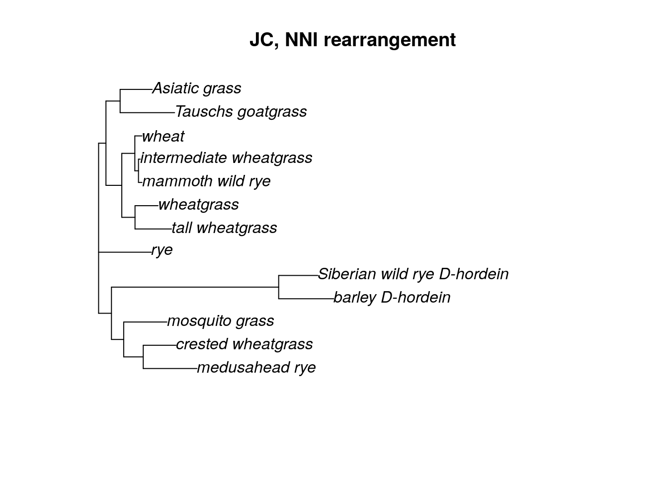
With the choice of NNI rearrangement, you can see that only a few moves were necessary in order to find the ML tree. We can also choose a “stochastic” or “ratchet” (likelihood ratchet) tree rearrangement algorithm. I like to use the stochastic rearrangement.
Using either the stochastic or ratchet tree rearrangement takes more time than NNI. Here I’ve also added a command to hide the output while the algorithm is running, but feel free to leave it off so you can see what the algorithm is doing!
fitJC <- optim.pml(fit, rearrangement = "stochastic", control = pml.control(trace = 0))
plot(fitJC$tree, main = "JC, stochastic rearrangement")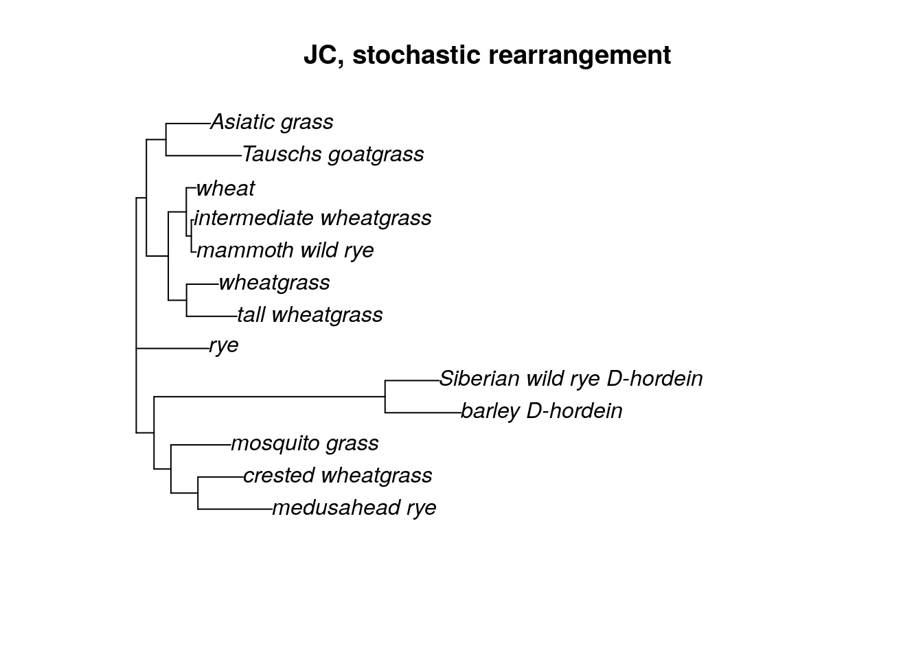
18.4 Changing the model for your ML search
All the work above is for the Jukes-Cantor model. However, there is a whole world of other substition models out there, and it would be nice to use them as well. We can update the pml object “fit” with other models.
According to the model test we ran on the grass data in the Neighbor Joining section, the best model for this dataset is the GTR + G model. The gamma distribution has two parameters, a shape parameter and a scale parameter. In phylogenetics, we commonly think of these as the number of rate categories and a shape parameter. When adding a gamma distribution, we can just specify the number of rate categories to start. The standard is 4.
## model: GTR+G(4)
## loglikelihood: -12503.04
## unconstrained loglikelihood: -20944.97
## Discrete gamma model
## Number of rate categories: 4
## Shape parameter: 1
##
## Rate matrix:
##   a c g t
## a 0 1 1 1
## c 1 0 1 1
## g 1 1 0 1
## t 1 1 1 0
##
## Base frequencies:
##    a    c    g    t
## 0.25 0.25 0.25 0.25
After we update the model and add the gamma distribution, we can see that fitGTR now 4 rate categories and a shape parameter = 1. However, the rate matrix and base frequencies are still the same as the JC model, because we did not update those. We could if we wanted to, but it’s easier to let the optim.pml algorithm do it.
fitGTR.G <- optim.pml(fitGTR.G, model = "GTR", optGamma = T, rearrangement = "stochastic", control = pml.control(trace = 0))

fitGTR.G
## model: GTR+G(4)
## loglikelihood: -11945.78
## unconstrained loglikelihood: -20944.97
## Discrete gamma model
## Number of rate categories: 4
## Shape parameter: 1.19688
##
## Rate matrix:
## a c g t
## a 0.0000000 0.4378420 1.6826685 0.7665308
## c 0.4378420 0.0000000 0.4612309 2.7050199
## g 1.6826685 0.4612309 0.0000000 1.0000000
## t 0.7665308 2.7050199 1.0000000 0.0000000
##
## Base frequencies:
## a c g t
## 0.3196529 0.2974113 0.2592177 0.1237181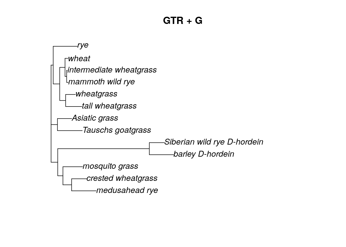
We can also update the model to include an invariant sites parameter (inv = 0.2).
fitGTR.G.I <- update(fitGTR.G, inv = 0.2)

fitGTR.G.I <- optim.pml(fitGTR.G.I, model = "GTR", optGamma = T, optInv = T,  rearrangement = "stochastic", control = pml.control(trace = 0))

fitGTR.G.I
## model: GTR+G(4)+I
## loglikelihood: -11945.78
## unconstrained loglikelihood: -20944.97
## Proportion of invariant sites: 5.218644e-05
## Discrete gamma model
## Number of rate categories: 4
## Shape parameter: 1.196526
##
## Rate matrix:
## a c g t
## a 0.0000000 0.4369734 1.6803296 0.7652394
## c 0.4369734 0.0000000 0.4602445 2.7015575
## g 1.6803296 0.4602445 0.0000000 1.0000000
## t 0.7652394 2.7015575 1.0000000 0.0000000
##
## Base frequencies:
## a c g t
## 0.3196556 0.2974835 0.2591984 0.1236624
Keep in mind that we never want to overwrite our original “fit” object. By updating the “fit” object (and saving the update by a new name), we can easily go back and change the model for our ML estimation. Let’s try a K80 (Kimura 2-parameter) model with an invariant sites parameter. In the optim.pml command, we can leave out the optGamma = T argument because we no longer have a gamma distribution included in the model.
fitK80.I <- update(fit, model = "K80", inv = 0.2)

fitK80.I <- optim.pml(fitK80.I, model = "K80", optInv = T,  rearrangement = "stochastic", control = pml.control(trace = 0))

fitK80.I
## model: K80+I
## loglikelihood: -12195.32
## unconstrained loglikelihood: -20944.97
## Proportion of invariant sites: 0.2632001
##
## Rate matrix:
## a c g t
## a 0.000000 1.000000 3.275521 1.000000
## c 1.000000 0.000000 1.000000 3.275521
## g 3.275521 1.000000 0.000000 1.000000
## t 1.000000 3.275521 1.000000 0.000000
##
## Base frequencies:
## a c g t
## 0.25 0.25 0.25 0.25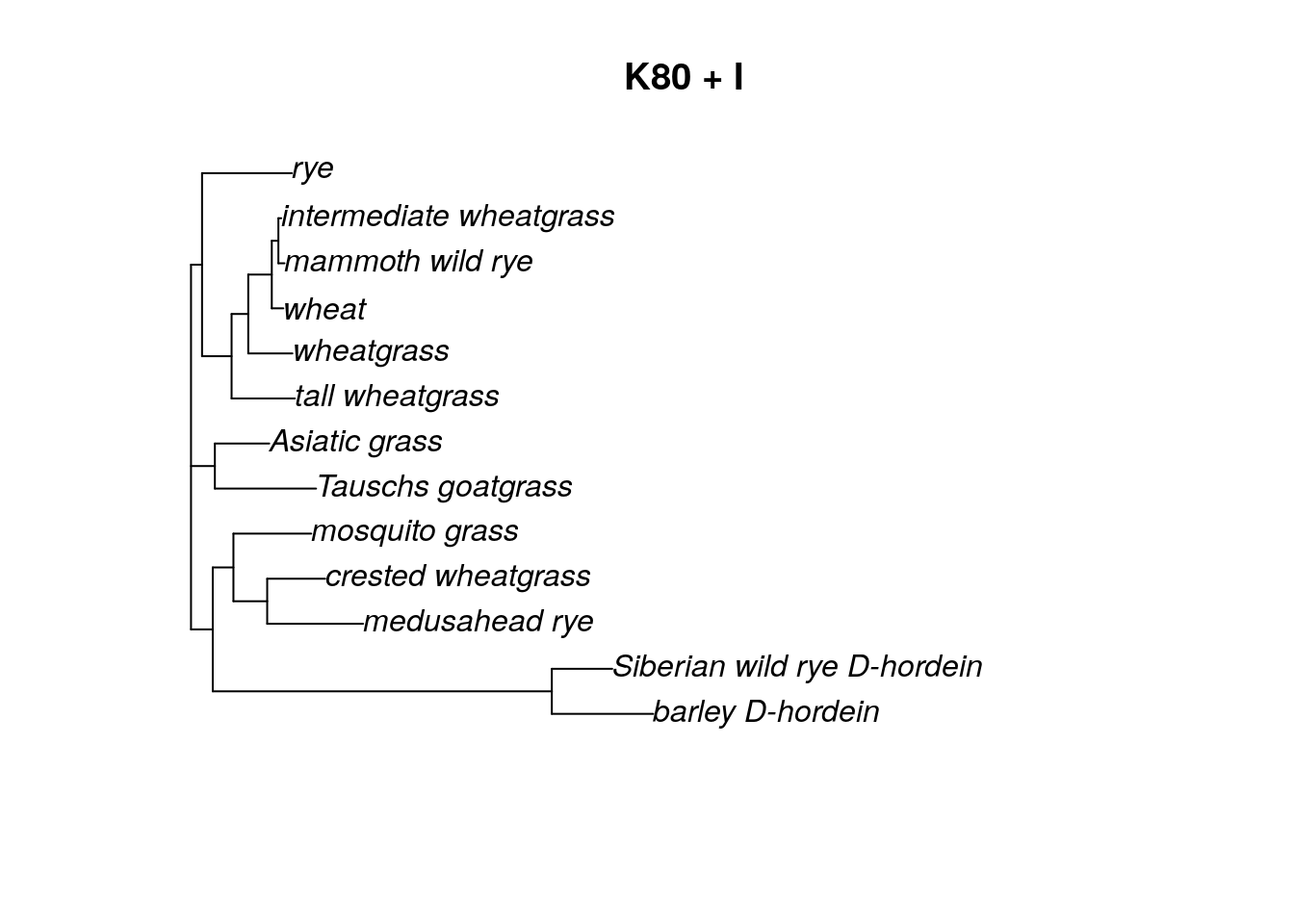
18.5 Bootstrapping the ML tree
Once we have decided which ML tree fits the data best (we can do so by choosing the one with the biggest log likelihood value), we can estimate the support for each branch in the tree with bootstrapping. Bootstrapping for ML trees can be very, very slow, so be patient!
Ideally we want to do at least 1000 bootstrap replicates. Many guides will set the number of bootstrap replicates to 100, but this is often chosen for speed. We really need at least 1000 replicates to have any sort of trust in the values.
We will use the bootstrap.pml command, which does have an option to estimate trees in parallel, which can help speed up the bootstrapping process. This option doesn’t appear to work on Windows machines, but it works fine on AnVIL. Using AnVIL itself will also help speed up the estimation.
Let’s try bootstrapping the GTR + G tree, which was the model chosen for us using the modelTest command.
bs <- bootstrap.pml(fitGTR.G, bs=1000, multicore = T, optNni=TRUE,
+ control = pml.control(trace = 0))To plot the bootstrap values, we can use a special plot function called plotBS. First, however, we need to root the tree. Then we can plot the rooted tree with our bootstrap values (saved in a list called “bs”), We are also going to format the bootstrap values so that only those values greater than 0.5 (50% bootstrap support) are shown using the p argument. We can also decide what color to make the bootstrap values and how many decimal places we want to see. (For a semi-complete list of colors in R, look here.)
tree.root <- root(fitGTR.G$tree, outgroup = c('barley_D-hordein','Siberian wild rye_D-hordein'))

plotBS(tree.root, bs, main = "GTR + G bootstrap", type = "p",
       bs.col="orange", p = 0.5, digits = 2)
18.6 Saving your bootstrap tree
Before you end your session, make sure to save your trees to your persistent disk.
## R version 4.3.2 (2023-10-31)
## Platform: x86_64-pc-linux-gnu (64-bit)
## Running under: Ubuntu 22.04.4 LTS
##
## Matrix products: default
## BLAS:   /usr/lib/x86_64-linux-gnu/openblas-pthread/libblas.so.3
## LAPACK: /usr/lib/x86_64-linux-gnu/openblas-pthread/libopenblasp-r0.3.20.so;  LAPACK version 3.10.0
##
## locale:
##  [1] LC_CTYPE=en_US.UTF-8       LC_NUMERIC=C
##  [3] LC_TIME=en_US.UTF-8        LC_COLLATE=en_US.UTF-8
##  [5] LC_MONETARY=en_US.UTF-8    LC_MESSAGES=en_US.UTF-8
##  [7] LC_PAPER=en_US.UTF-8       LC_NAME=C
##  [9] LC_ADDRESS=C               LC_TELEPHONE=C
## [11] LC_MEASUREMENT=en_US.UTF-8 LC_IDENTIFICATION=C
##
## time zone: Etc/UTC
## tzcode source: system (glibc)
##
## attached base packages:
## [1] stats     graphics  grDevices utils     datasets  methods   base
##
## other attached packages:
## [1] phangorn_2.11.1 ape_5.7-1
##
## loaded via a namespace (and not attached):
##  [1] sass_0.4.8       utf8_1.2.4       generics_0.1.3   xml2_1.3.6
##  [5] lattice_0.21-9   stringi_1.8.3    hms_1.1.3        digest_0.6.34
##  [9] magrittr_2.0.3   grid_4.3.2       evaluate_0.23    timechange_0.3.0
## [13] bookdown_0.41    fastmap_1.1.1    Matrix_1.6-1.1   rprojroot_2.0.4
## [17] jsonlite_1.8.8   processx_3.8.3   chromote_0.3.1   ps_1.7.6
## [21] promises_1.2.1   httr_1.4.7       fansi_1.0.6      ottrpal_1.3.0
## [25] codetools_0.2-19 jquerylib_0.1.4  cli_3.6.2        rlang_1.1.4
## [29] cachem_1.0.8     yaml_2.3.8       parallel_4.3.2   tools_4.3.2
## [33] tzdb_0.4.0       dplyr_1.1.4      fastmatch_1.1-4  vctrs_0.6.5
## [37] R6_2.5.1         lifecycle_1.0.4  lubridate_1.9.3  snakecase_0.11.1
## [41] stringr_1.5.1    janitor_2.2.0    pkgconfig_2.0.3  pillar_1.9.0
## [45] bslib_0.6.1      later_1.3.2      glue_1.7.0       Rcpp_1.0.12
## [49] highr_0.11       xfun_0.48        tibble_3.2.1     tidyselect_1.2.0
## [53] knitr_1.48       igraph_2.0.2     nlme_3.1-164     htmltools_0.5.7
## [57] websocket_1.4.2  rmarkdown_2.25   webshot2_0.1.1   readr_2.1.5
## [61] compiler_4.3.2   quadprog_1.5-8   askpass_1.2.0    openssl_2.1.1