
Chapter 5 Using Notebooks
5.1 Learning Objectives
Notebooks are a handy way to have the code, output, and scientist’s thought process all documented in one place that is easy for others to read and follow.
The notebook environment is incredibly useful for reproducible data science for a variety of reasons:
5.1.0.1 Reason 1: Notebooks allow for tracking data exploration and encourage the scientist to narrate their thought process:
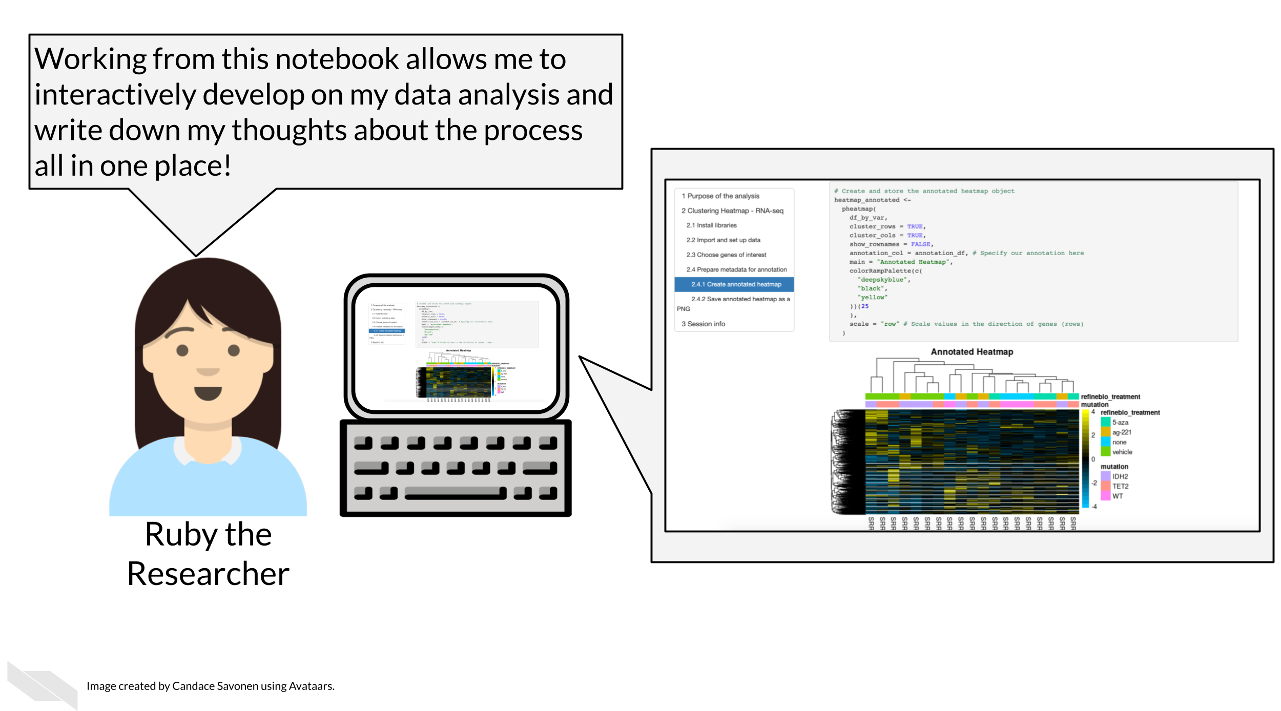
Each executed code cell is an attempt by the researcher to achieve something and to tease out some insight from the data set. The result is displayed immediately below the code commands, and the researcher can pause and think about the outcome. As code cells can be executed in any order, modified and re-executed as desired, deleted and copied, the notebook is a convenient environment to iteratively explore a complex problem.
5.1.0.2 Reason 2: Notebooks allow for easy sharing of results:

Notebooks can be converted to html and pdf, and then shared as static read-only documents. This is useful to communicate and share a study with colleagues or managers. By adding sufficient explanation, the main story can be understood by the reader, even if they wouldn’t be able to write the code that is embedded in the document.
5.1.0.3 Reason 3: Notebooks can be re-ran as a script or developed interactively:
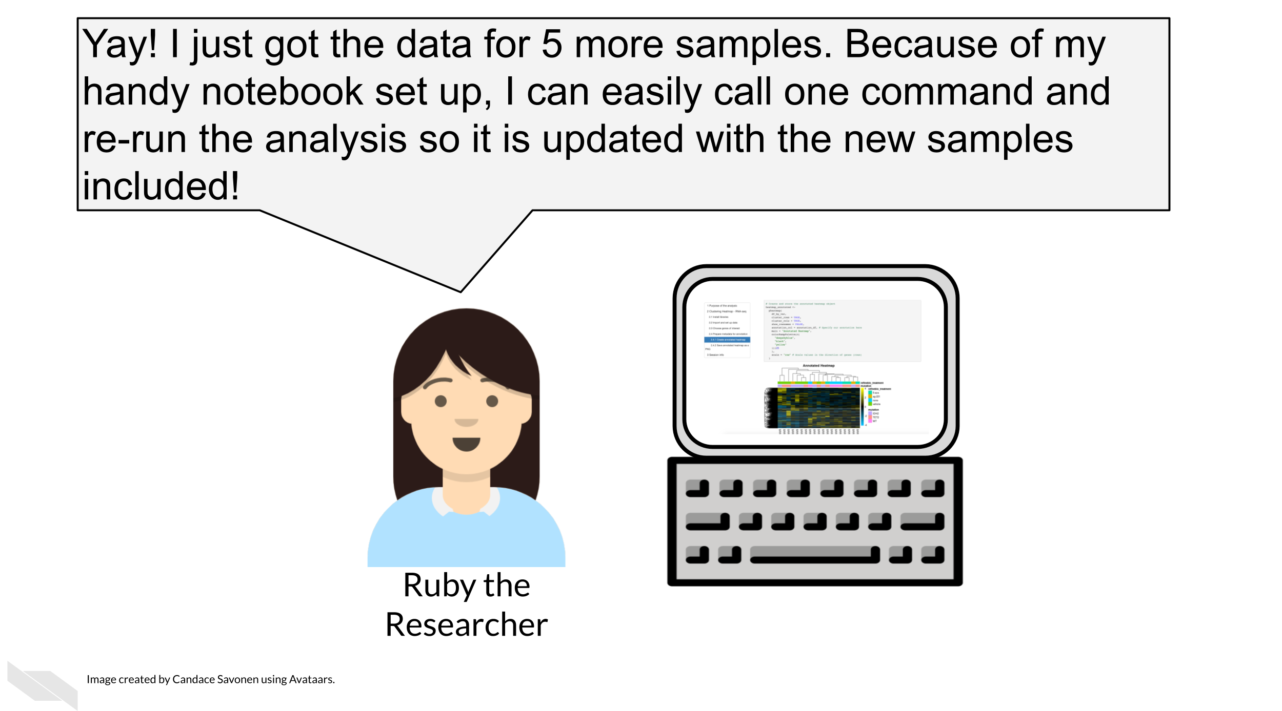
A common pattern in science is that a computational recipe is iteratively developed in a notebook. Once this has been found and should be applied to further data sets (or other points in some parameter space), the notebook can be executed like a script, for example by submitting these scripts as batch jobs.
This can also be handy especially if you use automation to enhance the reproducibility of your analyses (something we will talk about in the advanced part of this course).
Because of all of these reasons, we encourage the use of computational notebooks as a means of enhancing reproducibility. (This course itself is also written with the use of notebooks!)
5.2 Get the exercise project files
Get the Python project example files
Now double click your chapter zip file to unzip. For Windows you may have to follow these instructions.
Get the R project example files
Now double click your chapter zip file to unzip. For Windows you may have to follow these instructions.
5.3 Exercise: Convert code into a notebook!
5.3.1 Set up your IDE
For this chapter, we will create notebooks from our example files code. Notebooks work best with the integrated development environment (IDE) they were created to work with. IDE’s are sets of tools that help you develop your code. They are part “point and click” and part command line and include lots of visuals that will help guide you.
Set up a Python IDE
Install JupyterLab
We advise using the
condamethod to install JupyterLab, because we will return to talk more aboutcondalater on, so if you don’t haveconda, you will need to install that first. We advise going withAnacondainstead ofminiconda. To install Anaconda you can download from here. Download the installer, and follow the installation prompts.Start up Anaconda navigator. On the home page choose
JupyterLaband clickInstall. This may take a few minutes.Now you should be able to click
LaunchunderneathJupyterLab. This will open up a page in your Browser withJupyterLab.
Getting familiar with JupyterLab’s interface
The JupyterLab interface consists of a main work area containing tabs of documents and activities, a collapsible left sidebar, and a menu bar. The left sidebar contains a file browser, the list of running kernels and terminals, the command palette, the notebook cell tools inspector, and the tabs list.
The menu bar at the top of JupyterLab has top-level menus that expose actions available in JupyterLab with their keyboard shortcuts. The default menus are:
File: actions related to files and directories
Edit: actions related to editing documents and other activities
View: actions that alter the appearance of JupyterLab
Run: actions for running code in different activities such as notebooks and code consoles
Kernel: actions for managing kernels, which are separate processes for running code
Tabs: a list of the open documents and activities in the dock panel
Settings: common settings and an advanced settings editor
Help: a list of JupyterLab and kernel help links
Set up an R IDE
Install RStudio
- Install RStudio (and install R first if you have not already).
- After you’ve downloaded the RStudio installation file, double click on it and follow along with the installation prompts.
- Open up the RStudio application by double clicking on it.
Getting familiar with RStudio’s interface
The RStudio environment has four main panes, each of which may have a number of tabs that display different information or functionality. (their specific location can be changed under Tools -> Global Options -> Pane Layout).
- The Editor pane is where you can write R scripts and other documents. Each tab here is its own document. This is your text editor, which will allow you to save your R code for future use. Note that change code here will not run automatically until you run it.
- The Console pane is where you can interactively run R code.
- There is also a Terminal tab here which can be used for running programs outside R on your computer
- The Environment pane primarily displays the variables, sometimes known as objects that are defined during a given R session, and what data or values they might hold.
- The Help viewer pane has several tabs all of which are pretty important:
- The Files tab shows the structure and contents of files and folders (also known as directories) on your computer.
- The Plots tab will reveal plots when you make them
- The Packages tab shows which installed packages have been loaded into your R session
- The Help tab will show the help page when you look up a function
- The Viewer pane will reveal compiled R Markdown documents
From Shapiro et al. (2021)
More reading about RStudio’s interface:
5.3.2 Create a notebook!
Now, in your respective IDE, we’ll turn our unreproducible scripts into notebooks. In the next chapter we will begin to dive into the code itself, but for now, we’ll get the notebook ready to go.
Set up a Python notebook
- Start a new notebook by going to
New>Notebook. - Then open up this chapter’s example code folder and open the
make-heatmap.pyfile.
- Create a new code chunk in your notebook.
- Now copy and paste all of the code from
make-heatmap.pyinto a new chunk. We will later break up this large chunk of code into smaller chunks that are thematic in the next chapter. - Save your
Untitled.ipynbfile as something that tells us what it will end up doing likemake-heatmap.ipynb.
For more about using Jupyter notebooks see this by Mike (2021).
Set up an R notebook
- Start a new notebook by going to
File>New File>R Notebook.
- Then open up this chapter’s example code folder and open the
make_heatmap.Rfile. - Practice creating a new chunk in your R notebook by clicking the
Code>Insert Chunkbutton on the toolbar or by pressingCmd+Option+I(in Mac) orCtrl + Alt + I(in Windows). (You can also manually type out the back ticks and{})
- Delete all the default text in this notebook but keep the header which is surrounded by
---and looks like:
title: "R Notebook"
output: html_notebook
You can feel free to change the title from R Notebook to something that better suits the contents of this notebook.
- Now copy and paste all of the code from
make_heatmap.Rinto a new chunk. We will later break up this large chunk of code into smaller chunks that are thematic in the next chapter.
- Save your
untitled.Rmdinto something that tells us what it will end up doing likemake-heatmap.Rmd.
- Notice that upon saving your
.Rmdfile, a new file.nb.htmlfile of the same name is created. Open that file and chooseview in Browser. If RStudio asks you to choose a browser, then choose a default browser.
- This shows the nicely rendered version of your analysis and snapshots whatever output existed when the
.Rmdfile was saved.
For more about using R notebooks see this by Xie, Allaire, and Grolemund (2018).
Now that you’ve created your notebook, you are ready to start polishing that code!
Any feedback you have regarding this exercise is greatly appreciated; you can fill out this form!