Chapter 6 Managing package versions

6.1 Learning Objectives

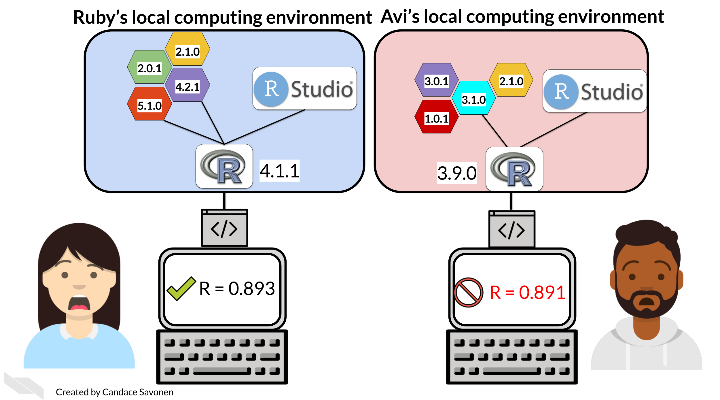
As we discussed previously, sometimes two different researchers can run the same code and same data and get different results!

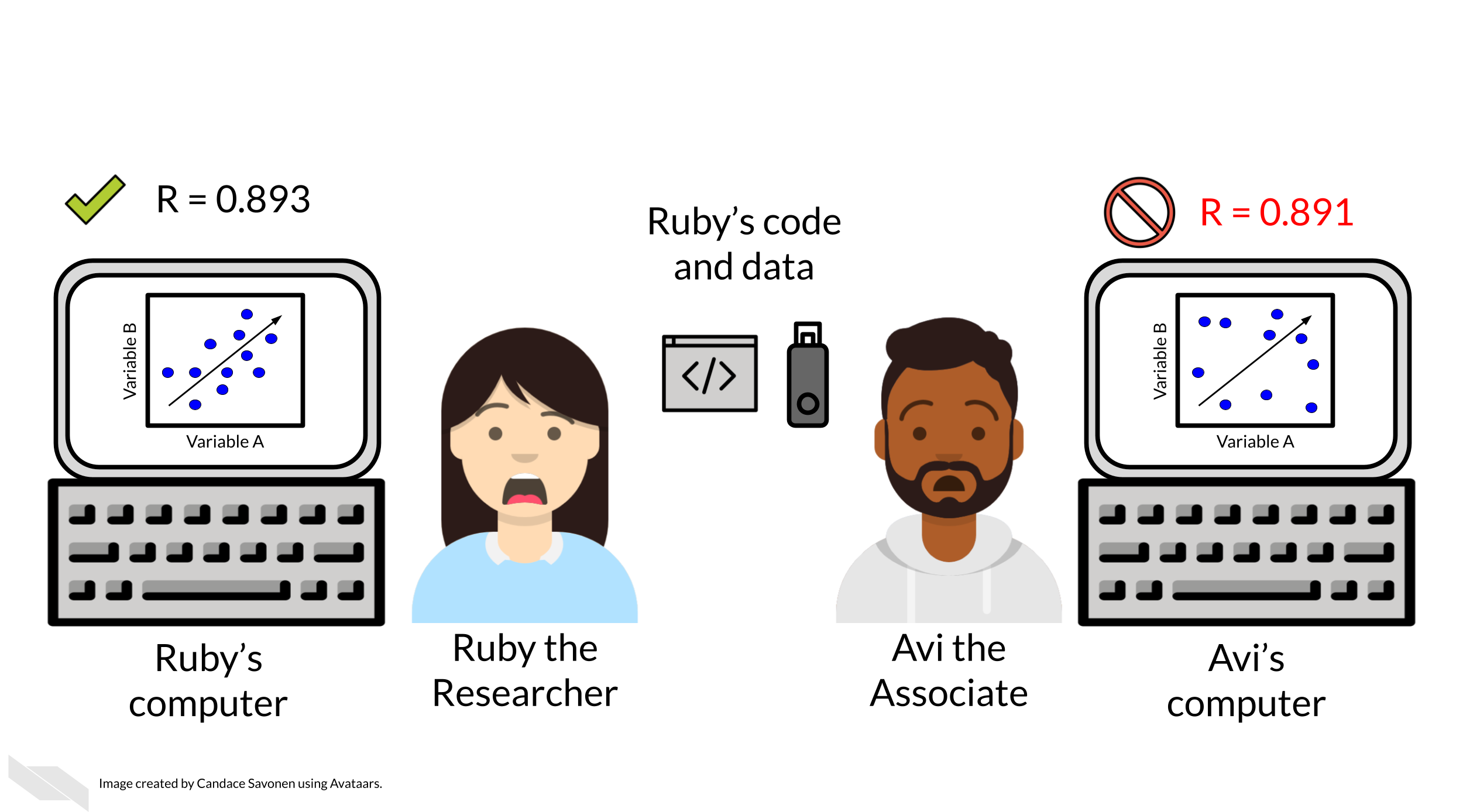
What Ruby and Avi may not realize is that although they may have used the same code and data, the software packages that they have on each of their computers might be very different. Even if they have the same software packages, they likely don’t have the same versions and versions can influence results! Different computing environments are not only a headache to detangle, they also can influence the reproducibility of your results (Beaulieu-Jones and Greene 2017).

There are multiple ways to deal with variations in computing environments so that your analyses will be reproducible and we will discuss a few different strategies for tackling this problem in this course and its follow up course. But for now, we will start with the least intensive to implement: session info.

There are two strategies for dealing with software versions that we will discuss in this chapter. Either of these strategies can be used alone or you can use both. They address different aspects of the computing environment discrepancy problem.

6.1.1 Strategy 1: Session Info - record a list of your packages

One strategy to combat different software versions is to list the session info. This is the easiest (though not most comprehensive) method for handling differences in software versions is to have your code list details about your computing environment.

Session info can lead to clues as to why results weren’t reproducible. For example, if both Avi and Ruby ran notebooks and included a session info print out it may look like this:

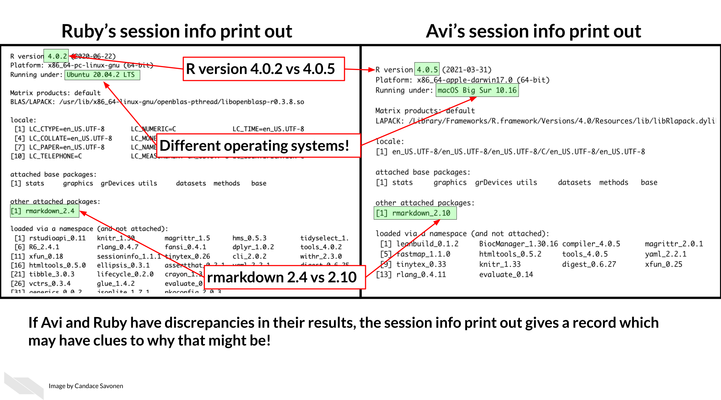
Session info shows us that they have different R versions and different operating systems. The packages they have attached is rmarkdown but they also have different rmarkdown package versions. If Avi and Ruby have discrepancies in their results, the session info print out gives a record which may have clues for any discrepancies. This can give them items to look into for determining why the results didn’t reproduce as expected.

6.1.2 Strategy 2: Package managers - share a useable snapshot of your environment

Package managers can help handle your computing environment for you in a way that you can share them with others. In general, package managers work by capturing a snapshot of the environment and when that environment snapshot is shared, it attempt to rebuild it. For R and Python versions of the exercises, we will be using different managers, but the foundational strategy will be the same: include a file that someone else could replicate your package set up from.

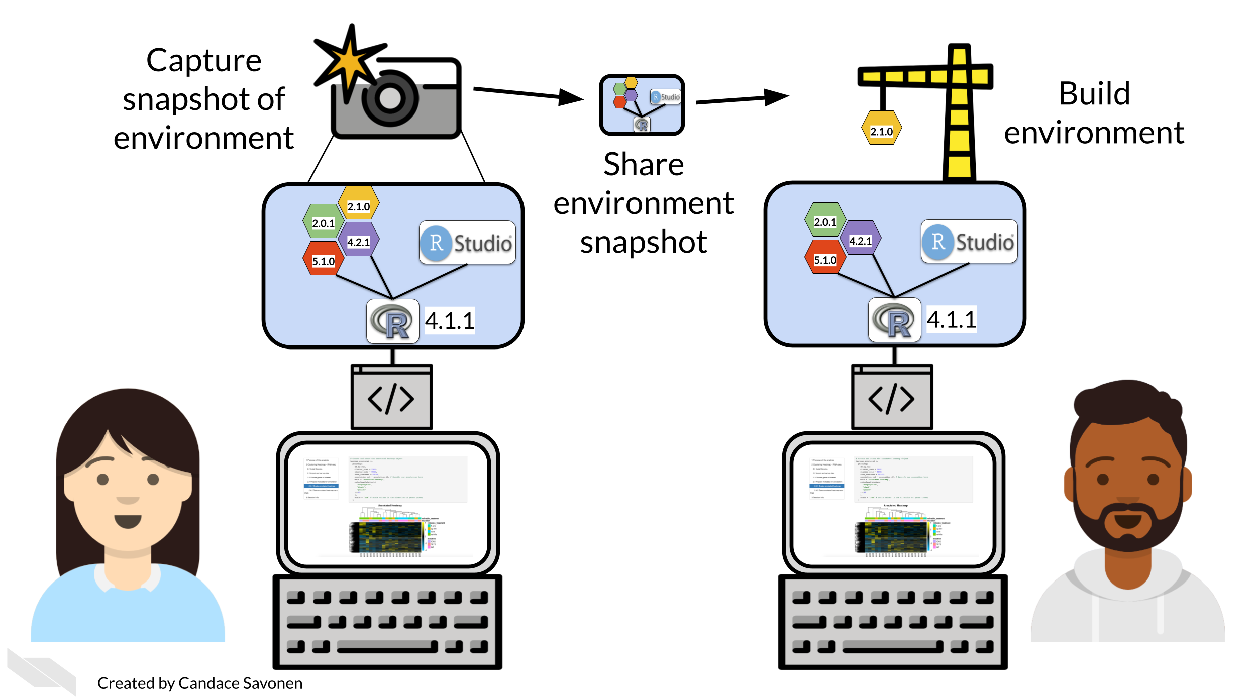
For both exercises, we will download an environment ‘snapshot’ file we’ve set up for you, then we will practice adding a new package to the environments we’ve provided, and add them to your new repository along with the rest of your example project files.

• For Python, we’ll use conda for package management and store this information in a environment.yml file.
• For R, we’ll use renv for package management and store this information in a renv.lock file.

6.2 Get the exercise project files (or continue with the files you used in the previous chapter)

Get the Python project example files

Click this link to download.

Now double click your chapter zip file to unzip. For Windows you may have to follow these instructions.

Get the R project example files

Click this link to download.

Now double click your chapter zip file to unzip. For Windows you may have to follow these instructions.

6.3 Exercise 1: Print out session info

Python version of the exercise

In your scientific notebook, you’ll need to add two items.
1. Add the import session_info to a code chunk at the beginning of your notebook.
2. Add session_info.show() to a new code chunk at the very end of your notebook.
2. Save your notebook as is. Note it will not run correctly until we address the issues with the code in the next chapter.

R version of the exercise

1. In your Rmd file, add a chunk in the very end that looks like this:

```r
sessionInfo()
```

```
## R version 4.0.2 (2020-06-22)
## Platform: x86_64-pc-linux-gnu (64-bit)
## Running under: Ubuntu 20.04.3 LTS
## 
## Matrix products: default
## BLAS/LAPACK: /usr/lib/x86_64-linux-gnu/openblas-pthread/libopenblasp-r0.3.8.so
## 
## locale:
##  [1] LC_CTYPE=en_US.UTF-8       LC_NUMERIC=C              
##  [3] LC_TIME=en_US.UTF-8        LC_COLLATE=en_US.UTF-8    
##  [5] LC_MONETARY=en_US.UTF-8    LC_MESSAGES=C             
##  [7] LC_PAPER=en_US.UTF-8       LC_NAME=C                 
##  [9] LC_ADDRESS=C               LC_TELEPHONE=C            
## [11] LC_MEASUREMENT=en_US.UTF-8 LC_IDENTIFICATION=C       
## 
## attached base packages:
## [1] stats     graphics  grDevices utils     datasets  methods   base     
## 
## loaded via a namespace (and not attached):
##  [1] knitr_1.33      magrittr_2.0.2  hms_0.5.3       R6_2.4.1       
##  [5] rlang_0.4.10    highr_0.8       stringr_1.4.0   httr_1.4.2     
##  [9] tools_4.0.2     xfun_0.26       jquerylib_0.1.4 htmltools_0.5.0
## [13] ellipsis_0.3.1  ottrpal_0.1.2   yaml_2.2.1      digest_0.6.25  
## [17] tibble_3.0.3    lifecycle_1.0.0 crayon_1.3.4    bookdown_0.24  
## [21] readr_1.4.0     vctrs_0.3.4     fs_1.5.0        curl_4.3       
## [25] evaluate_0.14   rmarkdown_2.10  stringi_1.5.3   compiler_4.0.2 
## [29] pillar_1.4.6    pkgconfig_2.0.3
```

2. Save your notebook as is. Note it will not run correctly until we address the issues with the code in the next chapter.

6.4 Exercise 2: Package management

Python version of the exercise

1. Download this starter conda environment.yml file by clicking on the link and place it with your example project files directory.

2. Navigate to your example project files directory using command line.

3. Create your conda environment by using this file in the command.

conda env create --file environment.yml

4. Activate your conda environment using this command.

conda activate reproducible-python

5. Now start up JupyterLab again using this command:

jupyter lab

6. Follow these instructions to add the environment.yml file to the GitHub repository you created in the previous chapter. Later we will practice and discuss how to more fully utilize the features of GitHub but for now, just drag and drop it as the instructions linked describe.

6.4.1 More resources on how to use conda

• Install Jupyter using your own environment (Mac specific)
• Definitive guide to using conda

R version of the exercise

First install the renv package

1. Go to RStudio and the Console pane:

2. Install renv using (you should only need to do this once per your computer or RStudio environment).

install.packages("renv")

Now set up renv to use in your project

1. Change to your current directory for your project using setwd() in your console window (don’t put this in a script or notebook).

2. Use this command in your project:

renv::init()

This will start up renv in your particular project

*What’s :: about? – in brief it allows you to use a function from a package without loading the entire thing with library().

3. Now you can develop your project as you normally would; installing and removing packages in R as you see fit. For the purposes of this exercise, let’s install the styler package using the following command. (The styler package will come in handy for styling our code in the next chapter).

install.packages("styler")

Now that we have installed styler we will want to add it to our renv snapshot.

4. To add any packages we’ve installed to our renv snapshot we will use this command:

renv::snapshot()

This will save whatever packages we are currently using to our environment snapshot file called renv.lock. This renv.lock file is what we can share with our collaborators so they can replicate our computing environment.

If your package installation attempts are unsuccessful and you’d like to revert to the previous state of your environment, you can run renv::restore(). This will restore your renv.lock file to what it was before you attempted to install styler or whatever packages you tried to install.

5. You should see an renv.lock file is now created or updated! You will want to always include this file with your project files. This means we will want to add it to our GitHub!

6. Follow these instructions to add your renv.lock file to the GitHub repository you created in the previous chapter. Later we will practice and discuss how to more fully utilize the features of GitHub but for now, just drag and drop it as the instructions linked describe.

After you’ve added your computing environment files to your GitHub, you’re ready to continue using them with your IDE to actually work on the code in your notebook!

Any feedback you have regarding this exercise is greatly appreciated; you can fill out this form!