Chapter 7 Marker gene detection

We have managed to identify clusters of related cells in the data. However, these clusters aren’t very useful until we can identify the biology meaning of each group. This is where functional annotation comes in.

The real art, and the greatest challenge, in an scRNA-seq analysis comes when interpreting the results. Up to this point (cleaning and clustering the data), the analysis and computation has been straightforward. Figuring out the biological state that each cluster represents, on the other hand, is more difficult, as it requires applying prior biological knowledge to the dataset.

Thanks to previous research, we know many marker genes, or genes can be used to identify particular cell types. These genes are differentially expressed across cell types, and by examining the expression profiles of multiple marker genes across all the clusters, we can assign particular cell type identities to each cluster.

7.1 Calculating and ranking effect size summary statistics

We begin by comparing each pair of clusters and calculating scores for expression differences between the two for each gene. We have multiple options for the statistics used to compare expression values.

AUC (area under the curve) is the probability that a randomly chosen observation from cluster A is greater than a randomly chosen observation from cluster B. This statistic is a way to quantify how well we can distinguish between two distributions (clusters) in a pairwise comparison. An AUC of 1 means all values in cluster A are greater than any value from cluster B and suggests upregulation. An AUC of of 0.5 means the two clusters are indistinguishable from each other, while an AUC of 0 suggests the marker gene observations in cluster A are downregulated compared to those in cluster B.
Cohen’s d is a standardized log-fold change, and can be thought of as the number of standard deviations that separate the two groups. Positive values of Cohen’s d suggest that our cluster of interest (cluster A) are upregulated compared to cluster B, while negative values suggest the marker gene observations in cluster A are downregulated compared to cluster B.
log-fold change (logFC) is a measure of whether there is a difference in expression between clusters. Keep in mind that these values ignore the magnitude of the change. As with the others, positive values indicate upregulation in the cluster of interest (cluster A), while negative values indicate downregulation.

For each of these statistics, scoreMarkers calculates mean, median, minimum value (min), maximum value (max), and minimum rank (rank; the smallest rank of each gene across all pairwise comparisons). For most of these measures, a larger number indicates upregulation. For minimum rank, however, a small value means the gene is one of the top upregulated genes.

AUC or Cohen’s d are effective regardless of the magnitude of the expression values and thus are good choices for general marker detection. The log-fold change in the detected proportion is specifically useful for identifying binary changes in expression.

For this exercise, we’re going to focus on upregulated markers, since those are particularly useful for identifying cell types in a heterogeneous population like the Zeisel dataset. We use the findMarkers command, which quickly identifies potential marker genes.

# identify those genes which are upregulated in some clusters compared to others
markers <- findMarkers(sce.zeisel.tsne20, direction = "up")
marker.set <- markers[["1"]]
head(marker.set, 10)

## DataFrame with 10 rows and 18 columns
##               Top      p.value          FDR summary.logFC   logFC.2   logFC.3
##         <integer>    <numeric>    <numeric>     <numeric> <numeric> <numeric>
## Syngr3          1 5.71433e-140 1.90535e-137       2.44603  1.156187 1.1330628
## Mllt11          1 3.31857e-249 7.37681e-246       2.87647  0.971725 1.4504728
## Ndrg4           1  0.00000e+00  0.00000e+00       3.83936  1.146289 0.9309904
## Slc6a1          1 1.75709e-160 8.57373e-158       3.46313  3.063161 3.2821288
## Gad1            1 4.70797e-234 8.56251e-231       4.54282  4.024699 4.3901265
## Gad2            1 1.32400e-208 1.76586e-205       4.24931  3.756435 3.9505814
## Atp1a3          1 3.54623e-279 1.41892e-275       3.45285  1.213985 0.0213418
## Slc32a1         2 1.50335e-109 2.48562e-107       1.91750  1.791641 1.8496954
## Rcan2           2 9.25451e-129 2.50197e-126       2.21812  1.432185 2.1127708
## Rab3a           2 1.61475e-202 1.61523e-199       2.52266  0.884615 0.6329209
##           logFC.4   logFC.5   logFC.6   logFC.7   logFC.8   logFC.9  logFC.10
##         <numeric> <numeric> <numeric> <numeric> <numeric> <numeric> <numeric>
## Syngr3    2.38928   2.44603 0.7085503 0.8470822  1.159959  2.525116  1.030908
## Mllt11    2.94289   2.87647 0.4897958 0.0882716  1.030983  3.262597  0.471414
## Ndrg4     3.67150   3.83936 0.3680955 0.7169171  1.103046  3.646328  0.791827
## Slc6a1    2.92969   2.88778 3.6063318 3.5292982  2.218826  0.704948  3.571574
## Gad1      4.37025   4.46268 4.6478826 4.5428243  4.477666  4.386587  4.572889
## Gad2      4.08621   4.15971 4.2916168 4.2222656  4.229715  4.207704  4.249309
## Atp1a3    3.18678   3.45285 0.6498389 0.1656598  0.426762  3.436859 -0.228370
## Slc32a1   1.93798   1.91658 1.9393715 1.9092434  1.913338  1.917505  1.910826
## Rcan2     1.81884   1.25488 1.1051970 2.1730716  2.170402  2.102633  2.218119
## Rab3a     2.73747   2.52266 0.0267138 0.3133349  0.695216  2.921335  0.163635
##          logFC.11  logFC.12  logFC.13  logFC.14  logFC.15
##         <numeric> <numeric> <numeric> <numeric> <numeric>
## Syngr3   0.684417   2.56482   2.55195   2.58830   2.42180
## Mllt11   0.229326   3.04261   2.77725   3.08889   2.01497
## Ndrg4    0.565654   3.82140   4.14743   3.97144   4.01655
## Slc6a1   3.463131   3.43495   3.34170   3.05042   3.25178
## Gad1     4.568481   4.51547   4.50591   4.39482   4.63836
## Gad2     4.263975   4.16831   4.29808   4.09088   4.35014
## Atp1a3   1.118434   3.31854   3.78426   3.67087   3.60817
## Slc32a1  1.916869   1.94707   1.94707   1.94707   1.90680
## Rcan2    1.142480   2.09515   1.26318   1.46319   2.24552
## Rab3a    0.508261   3.16930   2.54753   3.06401   2.30063

This dataframe shows us the in log-fold expression change for each potential marker gene between cluster 1 and every other cluster.

7.2 Comparing gene expression levels across clusters

Once we’ve identified potential marker genes, we can use a heatmap to compare gene expression in each cell between clusters.

# pull the top-most upregulated markers from cluster 1 (compared to the rest of the clusters) and look at their expression in all clusters
top.markers <- rownames(marker.set)[marker.set$Top <= 10]
plotHeatmap(sce.zeisel.tsne20, features = top.markers, order_columns_by = "label")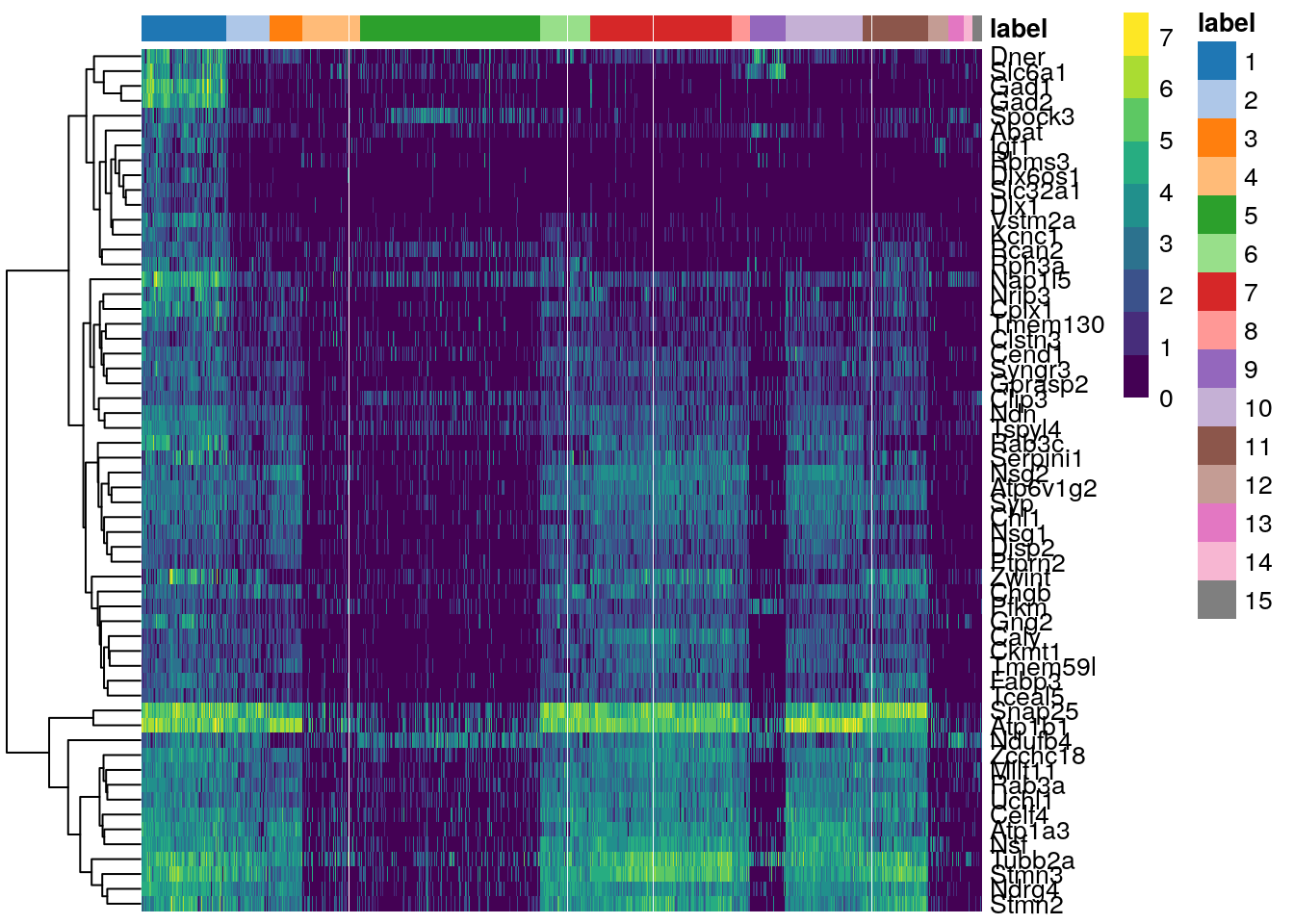

In this heatmap, clusters are on the horizontal, while the top upregulated genes in cluster 1 are on the vertical. The magnitude of the log-fold expression change is indicated by color of each cell.

We can also create a heatmap that shows the mean log-fold change of cluster 1 cells compared to the mean of each other cluster. This can simplify the heatmap and is useful when dealing with many clusters.

# AnVIL::install("pheatmap")
library(pheatmap)

#this heatmap lets us compare the average expression of the gene within a cluster compared to the other clusters
logFCs <- getMarkerEffects(marker.set[1:50,])
pheatmap(logFCs, breaks = seq(-5, 5, length.out = 101))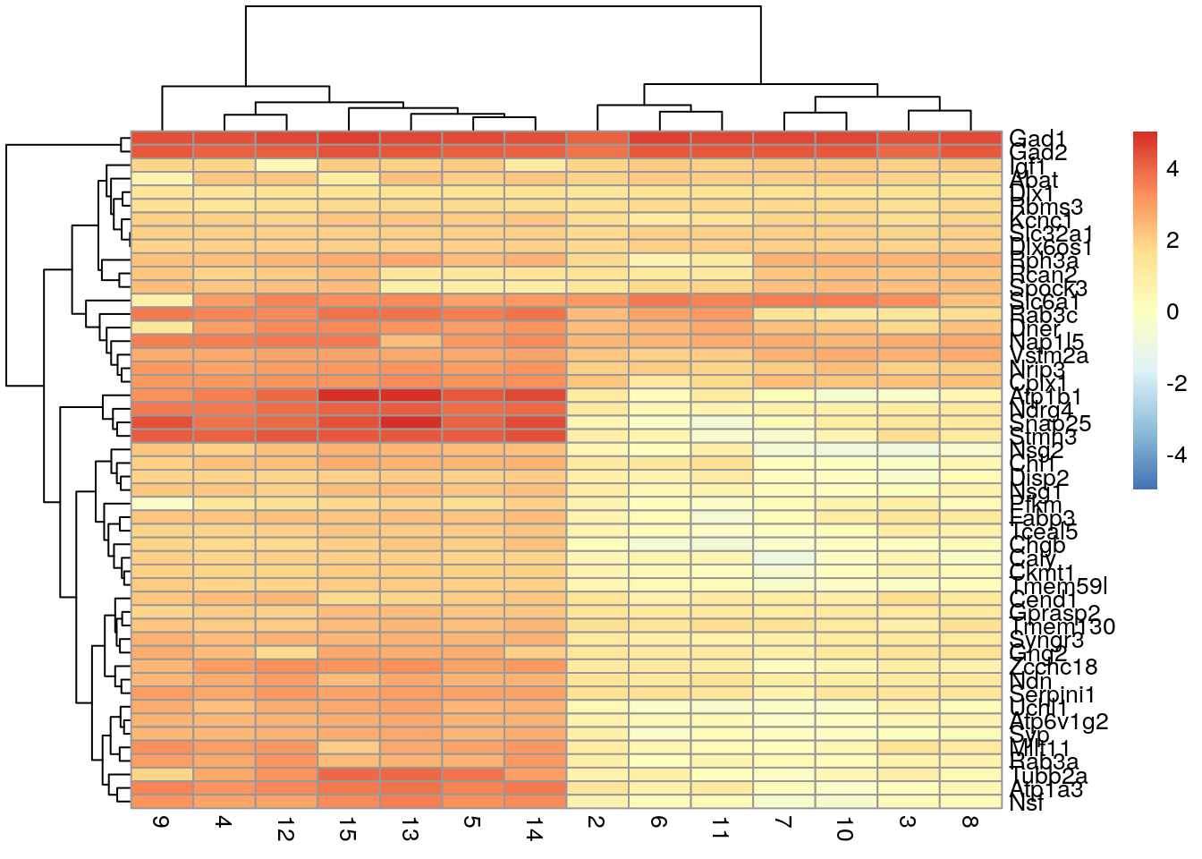

Here we see that three genes are generally upregulated in Cluster 1 compared to the other clusters: Gad1, Gad2, and Slc6a1. This is where prior biological knowledge comes in handy, as both Gad1 and Slc6a1 are known interneuron markers (Zeng et al. 2012).

QUESTION 1. Are there any groups or patterns you see in the second heatmap that look interesting?