
Chapter 4 Choosing features for the analysis
The goal with many scRNA-seq analyses is to identify differences in gene expression across multiple cell types; in order to do this, cells are clustered together into groups based on a single similarity (or dissimilarity) value between a pair of cells. Which genes you choose to include in the calculation of the similarity metric can greatly influence your downstream analyses.
In general, you will choose to include those genes with the greatest variability in gene expression across all the samples. The underlying assumption is this increased variability is “true” biological variation as opposed to technical noise.
4.1 Examining per-gene variation
We can calculate the per-gene variation across all samples using the variance of the log-normalized expression values you computed in the Normalization section. Because we are using a log-transformation, the total variance of a gene is partly driven by its abundance (not underlying biological heterogeneity). To correct for this relationship, we use a model that calculates the expected amount of variation for each abundance value. We then use the difference between the observed variation and the expected variation for each gene to identify highly-variable genes while controlling for cell abundance.
The Zeisel data was generated across multiple plates, so we need to be wary of any possible batch effects that could be driving highly-variable genes. Normally we would address this by blocking. However, each plate only contained 20-40 cells, and the cell population as a whole is highly heterogeneous, making it unlikely the sampled cell types on each plate is the same (one of the assumptions of blocking on plate). Thus, we will ignore blocking for this analysis.
If you work with a dataset that does not contain spike-ins, you would use the modelGeneVar() command instead of modelGeneVarWithSpikes().
# calculating per-gene variation for each samples using the log-normalized expression value; the "ERCC" option tells the algorithm that information about technical (that is, non-biological) variation can be calculated using the data column labeled "ERCC"
dec.zeisel.qc <- modelGeneVarWithSpikes(sce.zeisel.qc, "ERCC")

# plotting the expected variance (blue curve and orange points), as well as the observed variance (black points)
plot(dec.zeisel.qc$mean, dec.zeisel.qc$total, pch = 16, cex = 0.5,
    xlab = "Mean of log-expression", ylab = "Variance of log-expression")
curfit <- metadata(dec.zeisel.qc)
points(curfit$mean, curfit$var, col = "orange", pch = 16)
curve(curfit$trend(x), col = 'dodgerblue', add = TRUE, lwd = 2)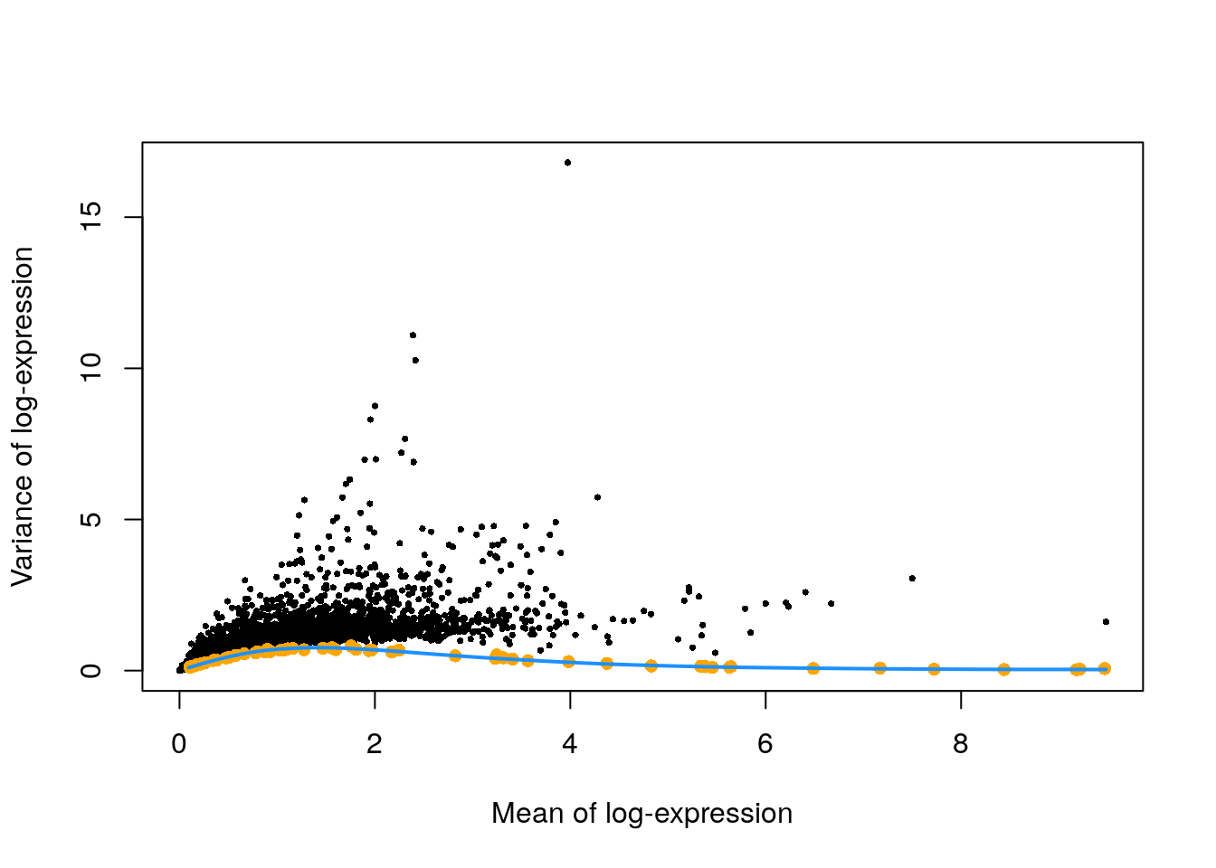
The expected variance for each log-expression value is plotted in orange. Observed values (the black points) much higher than this trend line will be used for downstream analyses.
4.2 Selecting highly variable genes
When choosing the genes for downstream analysis, you will need to balance choosing as many genes as possible (so as not to exclude important biological variation) with limiting the amount of random noise. The most straightforward approach is to simply take the top n genes after ranking based on the biological component of variance. We are creating objects with the top 500, 1000, and 2000 genes, so that we can examine how our choice of n impacts downstream calculations and steps.
# getting the top 500, 1000, and 2000 most-variable genes
top500.hvgs <- getTopHVGs(dec.zeisel.qc, n = 500)
top1000.hvgs <- getTopHVGs(dec.zeisel.qc, n = 1000)
top2000.hvgs <- getTopHVGs(dec.zeisel.qc, n = 2000)

# look at the cut-offs
dec.zeisel.qc <- dec.zeisel.qc[order(dec.zeisel.qc$bio, decreasing = TRUE),]
dec.zeisel.qc[c(1,500,1000,2000),1:6]
## DataFrame with 4 rows and 6 columns
## mean total tech bio p.value FDR
## <numeric> <numeric> <numeric> <numeric> <numeric> <numeric>
## Plp1 3.97379 16.80426 0.275699 16.528564 0.00000e+00 0.00000e+00
## Shfm1 2.64467 1.55363 0.534672 1.018959 5.54040e-47 2.04392e-45
## Cdc42 3.34431 1.04001 0.385442 0.654563 9.97095e-38 2.96239e-36
## Vdac2 1.81697 1.08138 0.720031 0.361348 7.90101e-05 2.55550e-04In this dataframe, the bio column represents the excess variation in gene expression (that is, the difference between the observed and expected expression). We are looking at four different genes - the gene with the greatest excess variation, as well as the last genes included in the top 500, top 1000, and top 2000 genes.
QUESTIONS
- What is the range of log-fold expression changes (the excess variation) when you choose the top 500 genes? What about when you choose the top 1000 genes? The top 2000 genes?
sessionInfo()## R version 4.1.3 (2022-03-10)
## Platform: x86_64-pc-linux-gnu (64-bit)
## Running under: Ubuntu 20.04.5 LTS
##
## Matrix products: default
## BLAS: /usr/lib/x86_64-linux-gnu/openblas-pthread/libblas.so.3
## LAPACK: /usr/lib/x86_64-linux-gnu/openblas-pthread/liblapack.so.3
##
## locale:
## [1] LC_CTYPE=en_US.UTF-8 LC_NUMERIC=C
## [3] LC_TIME=en_US.UTF-8 LC_COLLATE=en_US.UTF-8
## [5] LC_MONETARY=en_US.UTF-8 LC_MESSAGES=en_US.UTF-8
## [7] LC_PAPER=en_US.UTF-8 LC_NAME=C
## [9] LC_ADDRESS=C LC_TELEPHONE=C
## [11] LC_MEASUREMENT=en_US.UTF-8 LC_IDENTIFICATION=C
##
## attached base packages:
## [1] stats4 stats graphics grDevices utils datasets methods
## [8] base
##
## other attached packages:
## [1] scran_1.22.1 scater_1.22.0
## [3] ggplot2_3.3.5 scuttle_1.4.0
## [5] scRNAseq_2.8.0 SingleCellExperiment_1.16.0
## [7] SummarizedExperiment_1.24.0 Biobase_2.54.0
## [9] GenomicRanges_1.46.1 GenomeInfoDb_1.30.1
## [11] IRanges_2.28.0 S4Vectors_0.32.4
## [13] BiocGenerics_0.40.0 MatrixGenerics_1.6.0
## [15] matrixStats_0.61.0
##
## loaded via a namespace (and not attached):
## [1] AnnotationHub_3.2.2 BiocFileCache_2.2.1
## [3] igraph_1.3.1 lazyeval_0.2.2
## [5] BiocParallel_1.28.3 digest_0.6.29
## [7] ensembldb_2.18.4 htmltools_0.5.2
## [9] viridis_0.6.2 fansi_1.0.3
## [11] magrittr_2.0.3 memoise_2.0.1
## [13] ScaledMatrix_1.2.0 cluster_2.1.2
## [15] limma_3.50.3 Biostrings_2.62.0
## [17] prettyunits_1.1.1 colorspace_2.0-3
## [19] blob_1.2.3 rappdirs_0.3.3
## [21] ggrepel_0.9.1 xfun_0.26
## [23] dplyr_1.0.8 crayon_1.5.1
## [25] RCurl_1.98-1.6 jsonlite_1.8.0
## [27] glue_1.6.2 gtable_0.3.0
## [29] zlibbioc_1.40.0 XVector_0.34.0
## [31] DelayedArray_0.20.0 BiocSingular_1.10.0
## [33] scales_1.2.1 edgeR_3.36.0
## [35] DBI_1.1.2 Rcpp_1.0.8.3
## [37] viridisLite_0.4.0 xtable_1.8-4
## [39] progress_1.2.2 dqrng_0.3.0
## [41] bit_4.0.4 rsvd_1.0.5
## [43] metapod_1.2.0 httr_1.4.2
## [45] ellipsis_0.3.2 pkgconfig_2.0.3
## [47] XML_3.99-0.9 farver_2.1.0
## [49] sass_0.4.1 dbplyr_2.1.1
## [51] locfit_1.5-9.5 utf8_1.2.2
## [53] tidyselect_1.1.2 labeling_0.4.2
## [55] rlang_1.0.2 later_1.3.0
## [57] AnnotationDbi_1.56.2 munsell_0.5.0
## [59] BiocVersion_3.14.0 tools_4.1.3
## [61] cachem_1.0.6 cli_3.2.0
## [63] generics_0.1.2 RSQLite_2.2.12
## [65] ExperimentHub_2.2.1 evaluate_0.15
## [67] stringr_1.4.0 fastmap_1.1.0
## [69] yaml_2.3.5 knitr_1.33
## [71] bit64_4.0.5 purrr_0.3.4
## [73] KEGGREST_1.34.0 AnnotationFilter_1.18.0
## [75] sparseMatrixStats_1.6.0 mime_0.12
## [77] xml2_1.3.3 biomaRt_2.50.3
## [79] compiler_4.1.3 beeswarm_0.4.0
## [81] filelock_1.0.2 curl_4.3.2
## [83] png_0.1-7 interactiveDisplayBase_1.32.0
## [85] statmod_1.4.36 tibble_3.1.6
## [87] bslib_0.3.1 stringi_1.7.6
## [89] highr_0.9 GenomicFeatures_1.46.5
## [91] lattice_0.20-45 bluster_1.4.0
## [93] ProtGenerics_1.26.0 Matrix_1.4-0
## [95] vctrs_0.4.1 pillar_1.7.0
## [97] lifecycle_1.0.1 BiocManager_1.30.16
## [99] jquerylib_0.1.4 BiocNeighbors_1.12.0
## [101] bitops_1.0-7 irlba_2.3.5
## [103] httpuv_1.6.5 rtracklayer_1.54.0
## [105] R6_2.5.1 BiocIO_1.4.0
## [107] bookdown_0.24 promises_1.2.0.1
## [109] gridExtra_2.3 vipor_0.4.5
## [111] assertthat_0.2.1 rjson_0.2.21
## [113] withr_2.5.0 GenomicAlignments_1.30.0
## [115] Rsamtools_2.10.0 GenomeInfoDbData_1.2.7
## [117] parallel_4.1.3 hms_1.1.1
## [119] grid_4.1.3 beachmat_2.10.0
## [121] rmarkdown_2.10 DelayedMatrixStats_1.16.0
## [123] shiny_1.7.1 ggbeeswarm_0.6.0
## [125] restfulr_0.0.13