
Chapter 7 Design Matrices
7.1 Overview
When performing differential expression analysis on genomic data (such as RNA-seq experiments), scientists usually use linear models to determine the direction (did expression go up or down?) and magnitude (by how much?) of the change in expression. These scientists are interested in understanding the relationship between gene expression (the “response” variable”) and variables that affect expression, such as a treatment or cell type (“explanatory variable(s)”).
Design matrices are fundamental concepts in mathematics, statistics, and other domains, but their application to genomic data can introduce some complexity.
See this Bioconductor vignette for an excellent, in-depth look at design matrices.
7.2 Types of Models
The type of explanatory variables in our experiment will determine what our model looks like.
7.2.1 Regression: Continuous Variables
Continuous variables, or covariates, are numeric. This means that we could create a scatterplot comparing the covariate and expression. We could then imagine drawing a best fit line through those points to create our model. Law et al. (2020) state:
[Covariates] can be the age or weight of an individual, or other molecular or cellular phenotypes on a sample… For covariates, it is generally of interest to know the rate of change between the response and the covariate, such as “how much does the expression of a particular gene increase/decrease per unit increase in age?”. We can use a straight line to model, or describe, this relationship, which takes the form of
\[Expression = \beta_{0} + \beta_{1}age\]
where the line is defined by \(\beta_{0}\) the y-intercept and \(\beta_{1}\) the slope. In this model, the age covariate takes continuous, numerical values such as 0.8, 1.3, 2.0, 5.6, and so on.
These \(\beta\) values are known as parameters and are important for determining the impact of explanatory variables on expression.

7.2.2 Means: Categorical Variables
Categorical variables are discrete variables, or factors. We can think of these variables as “bins” that our samples fall into. Law et al. (2020) state:
[Factors] are often separated into those that are of a biological nature (e.g. disease status, genotype, treatment, cell-type) and those that are of a technical nature (e.g. experiment time, sample batch, handling technician, sequencing lane). Unique values within a factor are referred to as levels. For example, genotype as a factor may contain two levels, “wildtype” and “mutant”. Here, it is generally of interest to determine the expected or mean gene expression for each state or level of the factor. The relationship between gene expression and the factor can be described, or modeled, in the form of
\[Expression = \beta_{1}wildtype + \beta_{2}mutant\]
where \(\beta_{1}\) represents the mean gene expression for wildtype, and \(\beta_{2}\) represents the mean gene expression for mutant.
The “genotype” factor in this model is not numeric like “age” above, so the calculations work a bit differently. For any given sample, it can be either wildtype or mutant but not both. So, the values “wildtype” and “mutant” can only be zero (no) or one (yes). When a sample is mutant, “wildtype” = 0, and \(\beta_{1}\) drops out of the equation. Likewise, when a sample is wildtype, “mutant” = 0, and \(\beta_{2}\) drops out of the equation. This kind of model is called a means model.

7.2.3 Mean-Reference: Categorical Variables
You can also design categorical models with a “reference” value for comparison. Law et al. (2020) state:
An alternative parameterisation of the means model directly calculates the gene expression difference between mutant and wildtype. It does so by using one of the levels as a reference. Such a model is parameterised for the mean expression of the reference level (e.g. wildtype), and the rest of the levels are parameterised relative to the reference (e.g. the difference between mutant and wildtype). The relationship between gene expression and genotype is modeled in the form of
\[Expression = \beta_{1} + \beta_{2}mutant\]
where \(\beta_{1}\) represents the mean gene expression for wildtype, and \(\beta_{2}\) is the difference between means of mutant and wildtype
This kind of model can be really useful if you are interested in the difference between groups rather than the estimated parameters for the groups themselves. This kind of model is called a mean-reference model.

7.3 Making a Design Matrix
Law et al. (2020) use the following data to demonstrate how you might build a design matrix. This is a very simple example - in reality, we’d have many more genes being expressed.
df## expression mouse age group
## 1 2.38 MOUSE1 1 HEALTHY
## 2 2.85 MOUSE2 2 HEALTHY
## 3 3.60 MOUSE3 3 HEALTHY
## 4 4.06 MOUSE4 4 SICK
## 5 4.61 MOUSE5 5 SICK
## 6 5.04 MOUSE6 6 SICK7.3.1 Regression: Continuous Variables
Use the model.matrix() function to create the design matrix with the continuous variable “age”.
model.matrix( ~ df$age)## (Intercept) df$age
## 1 1 1
## 2 1 2
## 3 1 3
## 4 1 4
## 5 1 5
## 6 1 6
## attr(,"assign")
## [1] 0 1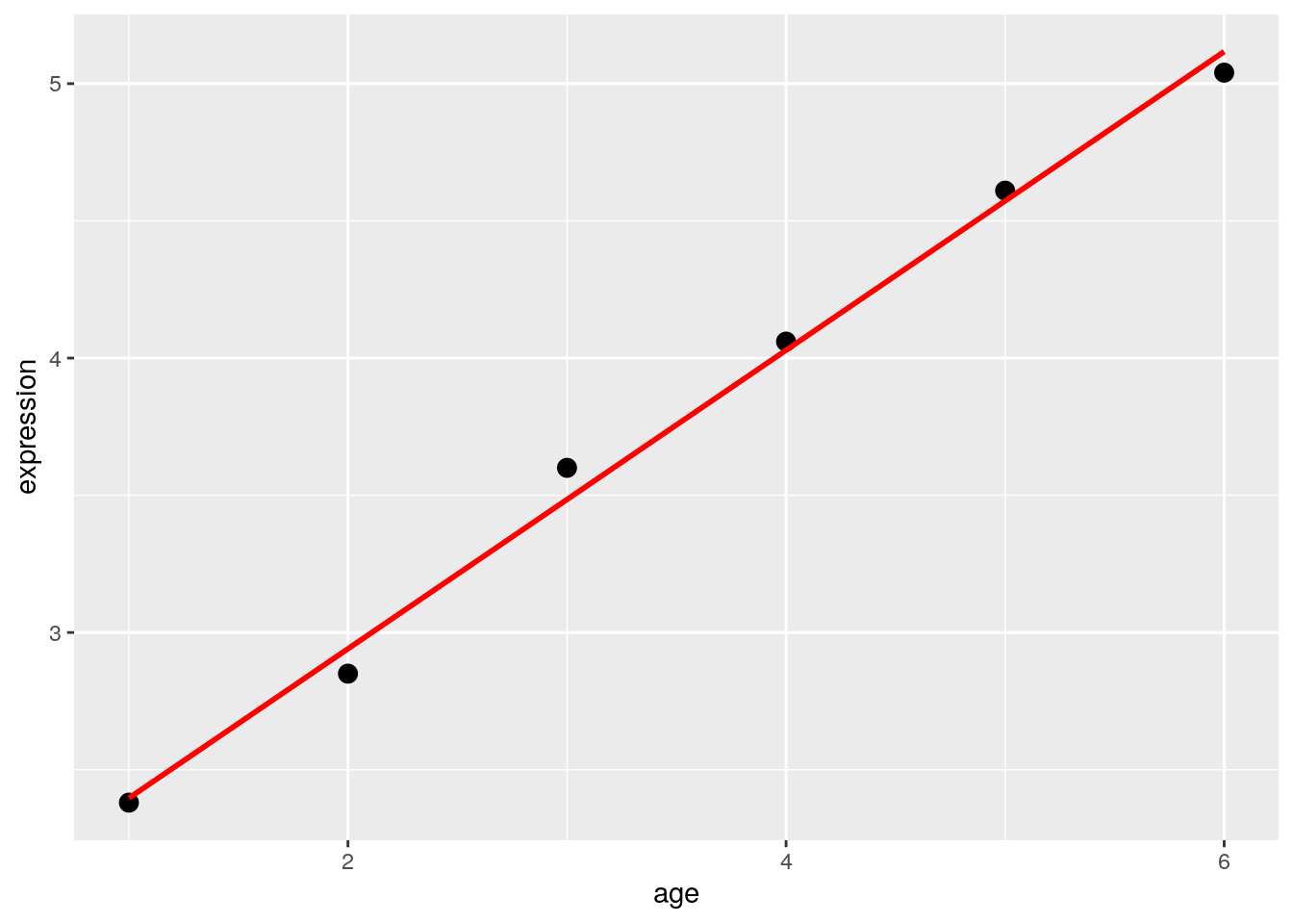
You can remove the intercept by adding zero to the design matrix. This forces the y-intercept to be zero. You could also use a different number here.
model.matrix( ~ 0 + df$age)## df$age
## 1 1
## 2 2
## 3 3
## 4 4
## 5 5
## 6 6
## attr(,"assign")
## [1] 1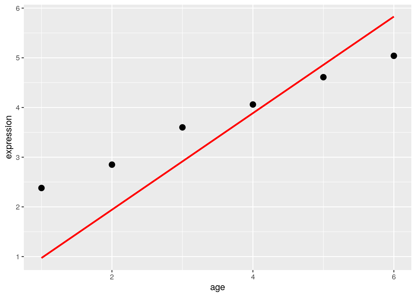
7.3.2 Means: Categorical Variables
Use the model.matrix() function to create the design matrix with the factor “group”. To create a means model, you should include a zero in the model.
model.matrix( ~ 0 + df$group)## df$groupHEALTHY df$groupSICK
## 1 1 0
## 2 1 0
## 3 1 0
## 4 0 1
## 5 0 1
## 6 0 1
## attr(,"assign")
## [1] 1 1
## attr(,"contrasts")
## attr(,"contrasts")$`df$group`
## [1] "contr.treatment"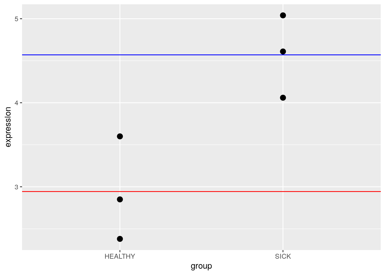
Notice that you only see zeros and ones for the two groups: df$groupHEALTHY and df$groupSICK.
7.3.3 Mean-Reference: Categorical Variables
Simply remove the zero to use a mean-reference model.
model.matrix( ~ df$group)## (Intercept) df$groupSICK
## 1 1 0
## 2 1 0
## 3 1 0
## 4 1 1
## 5 1 1
## 6 1 1
## attr(,"assign")
## [1] 0 1
## attr(,"contrasts")
## attr(,"contrasts")$`df$group`
## [1] "contr.treatment"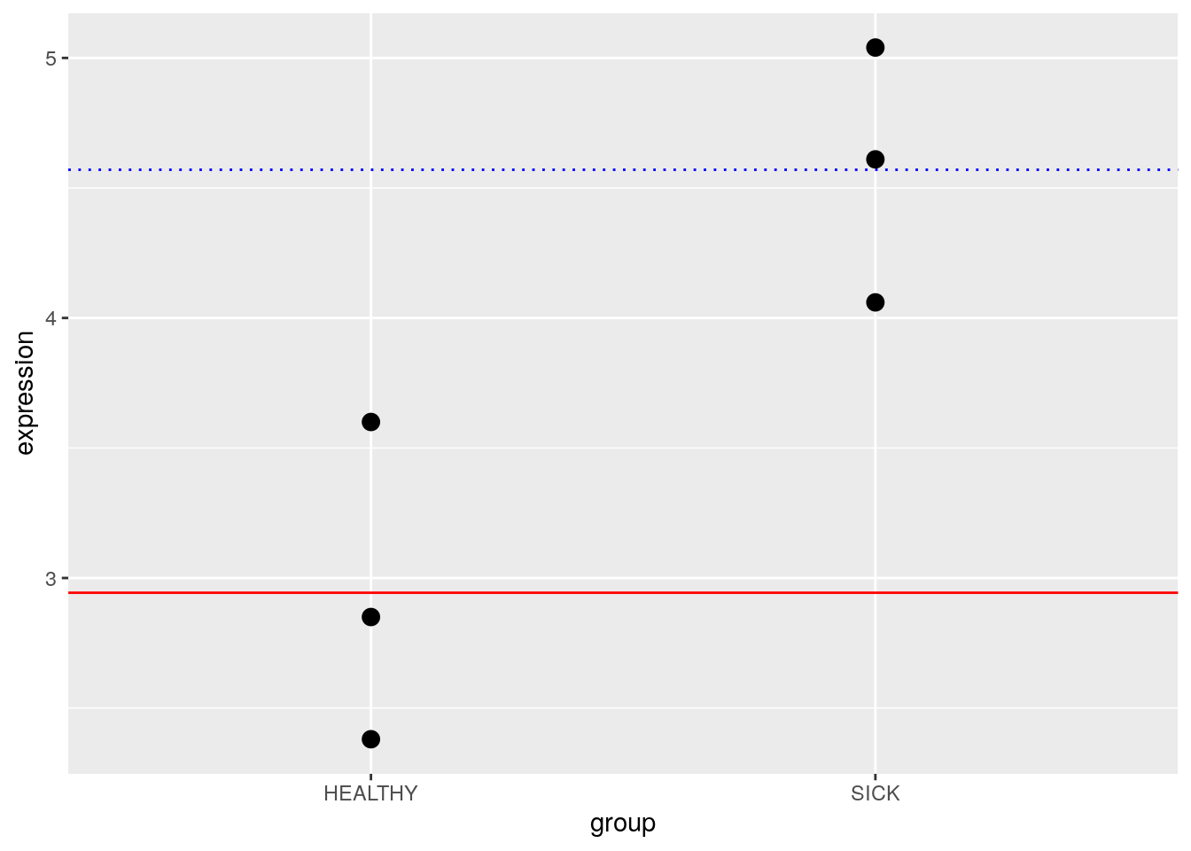
Notice how there is now an intercept. Remember that the parameter will now represent the difference between the groups instead of the second group mean.
7.4 More Complex Designs
model.matrix() can easily handle more complex experimental designs.
df2## expression mouse group type
## 1 2.38 MOUSE1 HEALTHY WILDTYPE
## 2 2.85 MOUSE2 HEALTHY WILDTYPE
## 3 3.60 MOUSE3 HEALTHY WILDTYPE
## 4 4.06 MOUSE4 SICK WILDTYPE
## 5 4.61 MOUSE5 SICK WILDTYPE
## 6 5.04 MOUSE6 SICK WILDTYPE
## 7 6.48 MOUSE7 HEALTHY MUTANT
## 8 6.70 MOUSE8 HEALTHY MUTANT
## 9 8.01 MOUSE9 HEALTHY MUTANT
## 10 11.99 MOUSE10 SICK MUTANT
## 11 12.81 MOUSE11 SICK MUTANT
## 12 14.73 MOUSE12 SICK MUTANTThe following will create a design matrix for “group” and “type”.
model.matrix( ~ df2$group + df2$type)## (Intercept) df2$groupSICK df2$typeWILDTYPE
## 1 1 0 1
## 2 1 0 1
## 3 1 0 1
## 4 1 1 1
## 5 1 1 1
## 6 1 1 1
## 7 1 0 0
## 8 1 0 0
## 9 1 0 0
## 10 1 1 0
## 11 1 1 0
## 12 1 1 0
## attr(,"assign")
## [1] 0 1 2
## attr(,"contrasts")
## attr(,"contrasts")$`df2$group`
## [1] "contr.treatment"
##
## attr(,"contrasts")$`df2$type`
## [1] "contr.treatment"Use the “*” to create a design matrix for the “group” and “type” as well as their interaction.
model.matrix( ~ df2$group + df2$type)## (Intercept) df2$groupSICK df2$typeWILDTYPE
## 1 1 0 1
## 2 1 0 1
## 3 1 0 1
## 4 1 1 1
## 5 1 1 1
## 6 1 1 1
## 7 1 0 0
## 8 1 0 0
## 9 1 0 0
## 10 1 1 0
## 11 1 1 0
## 12 1 1 0
## attr(,"assign")
## [1] 0 1 2
## attr(,"contrasts")
## attr(,"contrasts")$`df2$group`
## [1] "contr.treatment"
##
## attr(,"contrasts")$`df2$type`
## [1] "contr.treatment"7.5 Design Matrix in Practice
Let’s practice on a genomics dataset. Load the airway dataset. You might need to install it. Recall that the “airway” data is from an RNA-Seq experiment on four human airway smooth muscle cell lines treated with dexamethasone. You can learn more about the experiment in Himes (2014).
# AnVIL::install("airway")
library(airway)
data(airway)
In the SummarizedExperiment chapter, we learned that colData() provides descriptions of each sample.
colData(airway)## DataFrame with 8 rows and 9 columns
## SampleName cell dex albut Run avgLength
## <factor> <factor> <factor> <factor> <factor> <integer>
## SRR1039508 GSM1275862 N61311 untrt untrt SRR1039508 126
## SRR1039509 GSM1275863 N61311 trt untrt SRR1039509 126
## SRR1039512 GSM1275866 N052611 untrt untrt SRR1039512 126
## SRR1039513 GSM1275867 N052611 trt untrt SRR1039513 87
## SRR1039516 GSM1275870 N080611 untrt untrt SRR1039516 120
## SRR1039517 GSM1275871 N080611 trt untrt SRR1039517 126
## SRR1039520 GSM1275874 N061011 untrt untrt SRR1039520 101
## SRR1039521 GSM1275875 N061011 trt untrt SRR1039521 98
## Experiment Sample BioSample
## <factor> <factor> <factor>
## SRR1039508 SRX384345 SRS508568 SAMN02422669
## SRR1039509 SRX384346 SRS508567 SAMN02422675
## SRR1039512 SRX384349 SRS508571 SAMN02422678
## SRR1039513 SRX384350 SRS508572 SAMN02422670
## SRR1039516 SRX384353 SRS508575 SAMN02422682
## SRR1039517 SRX384354 SRS508576 SAMN02422673
## SRR1039520 SRX384357 SRS508579 SAMN02422683
## SRR1039521 SRX384358 SRS508580 SAMN02422677Notice above how the dex column indicates a trt or untrt condition. The following code will create a design matrix based on dex treatment. Since this is a categorical variable, we need to use a means or mean-reference model.
First, create a means model using the following code.
sample_data <- colData(airway)
model.matrix( ~ 0 + sample_data$dex)
## sample_data$dextrt sample_data$dexuntrt
## 1 0 1
## 2 1 0
## 3 0 1
## 4 1 0
## 5 0 1
## 6 1 0
## 7 0 1
## 8 1 0
## attr(,"assign")
## [1] 1 1
## attr(,"contrasts")
## attr(,"contrasts")$`sample_data$dex`
## [1] "contr.treatment"Now try creating a mean-reference model using the following.
model.matrix( ~ sample_data$dex)## (Intercept) sample_data$dexuntrt
## 1 1 1
## 2 1 0
## 3 1 1
## 4 1 0
## 5 1 1
## 6 1 0
## 7 1 1
## 8 1 0
## attr(,"assign")
## [1] 0 1
## attr(,"contrasts")
## attr(,"contrasts")$`sample_data$dex`
## [1] "contr.treatment"QUESTIONS:
- What is the difference between the two design matrices you created above?
- Does it matter which one you use? Why or why not?
7.6 Recap
sessionInfo()## R version 4.1.3 (2022-03-10)
## Platform: x86_64-pc-linux-gnu (64-bit)
## Running under: Ubuntu 20.04.5 LTS
##
## Matrix products: default
## BLAS: /usr/lib/x86_64-linux-gnu/openblas-pthread/libblas.so.3
## LAPACK: /usr/lib/x86_64-linux-gnu/openblas-pthread/liblapack.so.3
##
## locale:
## [1] LC_CTYPE=en_US.UTF-8 LC_NUMERIC=C
## [3] LC_TIME=en_US.UTF-8 LC_COLLATE=en_US.UTF-8
## [5] LC_MONETARY=en_US.UTF-8 LC_MESSAGES=en_US.UTF-8
## [7] LC_PAPER=en_US.UTF-8 LC_NAME=C
## [9] LC_ADDRESS=C LC_TELEPHONE=C
## [11] LC_MEASUREMENT=en_US.UTF-8 LC_IDENTIFICATION=C
##
## attached base packages:
## [1] stats4 stats graphics grDevices utils datasets methods
## [8] base
##
## other attached packages:
## [1] airway_1.14.0 SummarizedExperiment_1.24.0
## [3] Biobase_2.54.0 GenomicRanges_1.46.1
## [5] GenomeInfoDb_1.30.1 IRanges_2.28.0
## [7] S4Vectors_0.32.4 BiocGenerics_0.40.0
## [9] MatrixGenerics_1.6.0 matrixStats_0.61.0
## [11] ggplot2_3.3.5
##
## loaded via a namespace (and not attached):
## [1] lattice_0.20-45 png_0.1-7 assertthat_0.2.1
## [4] digest_0.6.29 utf8_1.2.2 R6_2.5.1
## [7] evaluate_0.15 httr_1.4.2 highr_0.9
## [10] pillar_1.7.0 zlibbioc_1.40.0 rlang_1.0.2
## [13] curl_4.3.2 jquerylib_0.1.4 Matrix_1.4-0
## [16] rmarkdown_2.10 labeling_0.4.2 splines_4.1.3
## [19] readr_2.1.2 stringr_1.4.0 RCurl_1.98-1.6
## [22] munsell_0.5.0 DelayedArray_0.20.0 compiler_4.1.3
## [25] xfun_0.26 pkgconfig_2.0.3 mgcv_1.8-39
## [28] htmltools_0.5.2 ottrpal_1.0.1 tidyselect_1.1.2
## [31] tibble_3.1.6 GenomeInfoDbData_1.2.7 bookdown_0.24
## [34] fansi_1.0.3 crayon_1.5.1 dplyr_1.0.8
## [37] tzdb_0.3.0 withr_2.5.0 bitops_1.0-7
## [40] grid_4.1.3 nlme_3.1-155 jsonlite_1.8.0
## [43] gtable_0.3.0 lifecycle_1.0.1 DBI_1.1.2
## [46] magrittr_2.0.3 scales_1.2.1 cli_3.2.0
## [49] stringi_1.7.6 farver_2.1.0 XVector_0.34.0
## [52] fs_1.5.2 bslib_0.3.1 ellipsis_0.3.2
## [55] generics_0.1.2 vctrs_0.4.1 tools_4.1.3
## [58] glue_1.6.2 purrr_0.3.4 hms_1.1.1
## [61] fastmap_1.1.0 yaml_2.3.5 colorspace_2.0-3
## [64] knitr_1.33 sass_0.4.1