pivot_longer()helps us take our data from wide to long formatnames_to =gives a new name to the pivoted columnsvalues_to =gives a new name to the values that used to be in those columns
pivot_wider()helps us take our data from long to wide formatnames_fromspecifies the old column name that contains the new column namesvalues_fromspecifies the old column name that contains new cell values
- to merge/join data sets together need a variable in common - usually “id”
Recap
Recap continued
- to merge/join data sets together need a variable in common - usually “id”
?join- see different types of joining fordplyrinner_join(x, y)- only rows that match forxandyare keptfull_join(x, y)- all rows ofxandyare keptleft_join(x, y)- all rows ofxare kept even if not merged withyright_join(x, y)- all rows ofyare kept even if not merged withxanti_join(x, y)- all rows fromxnot inykeeping just columns fromx.esquisser()function of theesquissepackage can help make plot sketches
esquisse and ggplot2
Why learn ggplot2?
More customization:
- branding
- making plots interactive
- combining plots
Easier plot automation (creating plots in scripts)
Faster (eventually)
ggplot2
A package for producing graphics - gg = Grammar of Graphics
Created by Hadley Wickham in 2005
Belongs to “Tidyverse” family of packages
“Make a ggplot” = Make a plot with the use of ggplot2 package
Resources:
ggplot2
Based on the idea of:
layering
plot objects are placed on top of each other with +
📉 +
📈
ggplot2

Slide Credit: Tanya Shapiro
ggplot2
Pros: extremely powerful/flexible – allows combining multiple plot elements together, allows high customization of a look, many resources online
Cons: ggplot2-specific “grammar of graphic” of constructing a plot

Artwork by @allison_horst. https://allisonhorst.com/
Tidy data
To make graphics using ggplot2, our data needs to be in a tidy format
Tidy data:
- Each variable forms a column.
- Each observation forms a row.
Messy data:
- Column headers are values, not variable names.
- Multiple variables are stored in one column.
- Variables are stored in both rows and columns.
Tidy data: example
Ideally we want each variable as a column and we want each observation in a row.
Column headers are values, not variable names:

Now the the data is “tidy” and in long format

Read more about tidy data and see other examples: Tidy Data tutorial
Data to plot
Type ?Orange for more information.
Is the data in tidy? Is it in long format?
head(Orange)
Tree age circumference 1 1 118 30 2 1 484 58 3 1 664 87 4 1 1004 115 5 1 1231 120 6 1 1372 142
First plot with ggplot2 package
First layer of code with ggplot2 package
Will set up the plot - it will be empty!

First layer of code with ggplot2 package
- Aesthetic mapping
aes(x= , y =)describes how variables in our data are mapped to elements of the plot - Note you don’t need to usemappingbut it is helpful to know what we are doing.
library(tidyverse) # don't forget to load ggplot2 (part of tidyverse)
# This is not code but shows the general format
ggplot({data_to plot}, aes(x = {var in data to plot},
y = {var in data to plot}))ggplot(Orange, aes(x = circumference, y = age))

Next layer code with ggplot2 package

There are many to choose from, to list just a few:
geom_point()– points (we have seen)geom_line()– lines to connect observationsgeom_boxplot()– boxplotsgeom_histogram()– histogramgeom_bar()– bar plotgeom_col()– column plotgeom_tile()– blocks filled with color
Next layer code with ggplot2 package
When to use what plot? A few examples:
- a scatterplot (
geom_point()): to examine the relationship between two sets of continuous numeric data - a barplot (
geom_bar()): to compare the distribution of a quantitative variable (numeric) between groups or categories - a histogram (
geom_hist()): to observe the overall distribution of numeric data - a boxplot (
geom_boxplot()): to compare values between different factor levels or categories
Next layer code with ggplot2 package
Need the + sign to add the next layer to specify the type of plot
ggplot({data_to plot}, aes(x = {var in data to plot},
y = {var in data to plot})) +
geom_{type of plot}</div>ggplot(Orange, aes(x = circumference, y = age)) + geom_point()

Read as: using Orange data, and provided aesthetic mapping, add points to the plot
Tip - plus sign + must come at end of line
Having the + sign at the beginning of a line will not work!
ggplot(food, aes(x = item_ID,
y = item_price_change,
fill = item_categ))
+ geom_boxplot()
Pipes will also not work in place of +!
ggplot(food, aes(x = item_ID,
y = item_price_change,
fill = item_categ)) %>%
geom_boxplot()
Plots can be assigned as an object
plt1 <- ggplot(Orange, aes(x = circumference, y = age)) +
geom_point()
plt1
Examples of different geoms
plt1 <- ggplot(Orange, aes(x = circumference, y = age)) +
geom_point()
plt2 <- ggplot(Orange, aes(x = circumference, y = age)) +
geom_line()
plt1 # fig.show = "hold" makes plots appear
plt2 # next to one another in the chunk settings


Specifying plot layers: combining multiple layers
Layer a plot on top of another plot with +
ggplot(Orange, aes(x = circumference, y = age)) + geom_point() + geom_line()

Adding color - can map color to a variable
ggplot(Orange, aes(x = circumference, y = age, color = Tree)) + geom_point() + geom_line()

Adding color - or change the color of each plot layer
You can change look of each layer separately. Note the arguments like linetype and alpha that allow us to change the opacity of the points and style of the line respectively.
ggplot(Orange, aes(x = circumference, y = age)) + geom_point(size = 5, color = "red", alpha = 0.5) + geom_line(size = 0.8, color = "black", linetype = 2)

linetype can be given as a number. See the docs for what numbers correspond to what linetype!
Customize the look of the plot

Customize the look of the plot
You can change the look of whole plot using theme_*() functions.
ggplot(Orange, aes(x = circumference, y = age)) + geom_point(size = 5, color = "red", alpha = 0.5) + geom_line(size = 0.8, color = "brown", linetype = 2) + theme_dark()

More themes!
There’s not only the built in ggplot2 themes but all kinds of themes from other packages!
Adding labels
The labs() function can help you add or modify titles on your plot. The title argument specifies the title. The x argument specifies the x axis label. The y argument specifies the y axis label.
ggplot(Orange, aes(x = circumference, y = age)) +
geom_point(size = 5, color = "red", alpha = 0.5) +
geom_line(size = 0.8, color = "brown", linetype = 2) +
labs(title = "My plot of orange tree data",
x = "Tree Circumference (mm)",
y = "Tree Age (days since 12/31/1968)")

Adding labels line break
Line breaks can be specified using \n within the labs() function to have a label with multiple lines.
ggplot(Orange, aes(x = circumference, y = age)) +
geom_point(size = 5, color = "red", alpha = 0.5) +
geom_line(size = 0.8, color = "brown", linetype = 2) +
labs(title = "Plot of orange tree data from 1968: \n trunk circumference vs tree age",
x = "Tree Circumference (mm)",
y = "Tree Age (days since 12/31/1968)")

Changing axis: specifying axis scale
scale_x_continuous() and scale_y_continuous() can change how the axis is plotted. Can use the breaks argument to specify how you want the axis ticks to be.
range(pull(Orange, circumference))
[1] 30 214
range(pull(Orange, age))
[1] 118 1582
plot_scale <-ggplot(Orange, aes(x = circumference, y = age)) +
geom_point(size = 5, color = "red", alpha = 0.5) +
geom_line(size = 0.8, color = "brown", linetype = 2) +
scale_x_continuous(breaks = seq(from = 20, to = 240, by = 20)) +
scale_y_continuous(breaks = seq(from = 100, to = 1600, by = 200))
Changing axis: specifying axis scale
plot_scale

ggplot(Orange, aes(x = circumference, y = age)) +
geom_point(size = 5, color = "red", alpha = 0.5) +
geom_line(size = 0.8, color = "brown", linetype = 2)

Changing axis: specifying axis limits
xlim() and ylim() can specify the limits for each axis
ggplot(Orange, mapping = aes(x = circumference, y = age)) + geom_point(size = 5, color = "red", alpha = 0.5) + geom_line(size = 0.8, color = "brown", linetype = 2) + labs(title = "My plot of orange tree circumference vs age") + xlim(100, max(pull(Orange, circumference)))

Modifying plot objects
You can add to a plot object to make changes! Note that we can save our plots as an object like plt1 below. And now if we reference plt1 again our plot will print out!
plt1 <- ggplot(Orange, aes(x = circumference, y = age)) + geom_point(size = 5, color = "red", alpha = 0.5) + geom_line(size = 0.8, color = "brown", linetype = 2) + labs(title = "My plot of orange tree circumference vs age") + xlim(100, max(pull(Orange, circumference))) plt1 + theme_minimal()

Overwriting specifications
It’s possible to go in and change specifications with newer layers
Orange %>% ggplot(aes(x = circumference,
y = age,
color = Tree)) +
geom_line(size = 0.8)

Overwriting specifications
It’s possible to go in and change specifications with newer layers
Orange %>% ggplot(aes(x = circumference,
y = age,
color = Tree)) +
geom_line(size = 0.8, color = "black")

GUT CHECK: If we get an empty plot what might we need to do?
A. Add a plot_ layer like plot_point()
B. Add a geom_ layer like geom_point()
GUT CHECK: How do we add more layers in ggplot2 plots?
A. %>%
B. &
C. +
Summary
ggplot()specifies what data use and what variables will be mapped to where- inside
ggplot(),aes(x = , y = , color =)specify what variables correspond to what aspects of the plot in general - layers of plots can be combined using the
+at the end of lines - special
theme_*()functions can change the overall look - individual layers can be customized using arguments like:
size,coloralpha(more transparent is closer to 0), andlinetype - labels can be added with the
labs()function andx,y,titlearguments - the\ncan be used for line breaks xlim()andylim()can limit or expand the plot areascale_x_continuous()andscale_y_continuous()can modify the scale of the axes- by default,
ggplot()removes points with missing values from plots.
Lab 1
💻 Lab
theme() function:
The theme() function can help you modify various elements of your plot. Here we will adjust the font size of the plot title.
ggplot(Orange, aes(x = circumference, y = age)) + geom_point(size = 5, color = "red", alpha = 0.5) + geom_line(size = 0.8, color = "brown", linetype = 2) + labs(title = "Circumference vs age") + theme(plot.title = element_text(size = 20))

theme() function
The theme() function always takes:
- an object to change (use
?theme()to see -plot.title,axis.title,axis.ticksetc.) - the aspect you are changing about this:
element_text(),element_line(),element_rect(),element_blank() - what you are changing:
- text:
size,color,fill,face,alpha,angle - position:
"top","bottom","right","left","none" - rectangle:
size,color,fill,linetype - line:
size,color,linetype
- text:
theme() function: center title and change size
The theme() function can help you modify various elements of your plot. Here we will adjust the horizontal justification (hjust) of the plot title.
ggplot(Orange, aes(x = circumference, y = age)) + geom_point(size = 5, color = "red", alpha = 0.5) + geom_line(size = 0.8, color = "brown", linetype = 2) + labs(title = "Circumference vs age") + theme(plot.title = element_text(hjust = 0.5, size = 20))

theme() function: change title and axis format
ggplot(Orange, aes(x = circumference, y = age)) +
geom_point(size = 5, color = "red", alpha = 0.5) +
geom_line(size = 0.8, color = "brown", linetype = 2) +
labs(title = "Circumference vs age") +
theme(plot.title = element_text(hjust = 0.5, size = 20),
axis.title = element_text(size = 16))

theme() function: moving (or removing) legend
If specifying position - use: “top”, “bottom”, “right”, “left”, “none”
ggplot(Orange, aes(x = circumference, y = age, color = Tree)) + geom_line() ggplot(Orange, aes(x = circumference, y = age, color = Tree)) + geom_line() + theme(legend.position = "none")


Cheatsheet about theme
https://github.com/claragranell/ggplot2/blob/main/ggplot_theme_system_cheatsheet.pdf

Keys for specifications
linetype

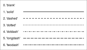
Linetype key
- geoms that draw lines have a
linetypeparameter - these include values that are strings like “blank”, “solid”, “dashed”, “dotdash”, “longdash”, and “twodash”
Orange %>% ggplot(aes(x = circumference,
y = age,
color = Tree)) +
geom_line(size = 0.8, linetype = "twodash")

Keys for specifications
shape

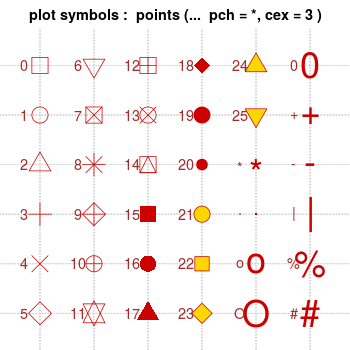
shape key
- geoms that draw have points have a
shapeparameter - these include numeric values (don’t need quotes for these) and some characters values (need quotes for these)
Orange %>% ggplot(aes(x = circumference,
y = age,
color = Tree)) +
geom_point(size = 2, shape = 12)

Can make your own theme to use on plots!
Guide on how to: https://rpubs.com/mclaire19/ggplot2-custom-themes
Group and/or color by variable’s values
First, we will read in some data for the purpose of demonstration about food prices over time.
food <- read_csv( file = "http://jhudatascience.org/intro_to_r/data/food_price.csv")
Food data
- 2 different categories (e.g. pasta, rice)
- 4 different items (e.g. 2 of each category)
- 10 price values changes collected over time for each item
food
# A tibble: 40 × 4 item_ID item_categ observation_time item_price_change <chr> <chr> <dbl> <dbl> 1 ID_1 pasta 1 1.5 2 ID_1 pasta 2 1.5 3 ID_1 pasta 3 0.5 4 ID_1 pasta 4 2.5 5 ID_1 pasta 5 0.5 6 ID_1 pasta 6 0.5 7 ID_1 pasta 7 1.5 8 ID_1 pasta 8 1.5 9 ID_1 pasta 9 2.5 10 ID_1 pasta 10 1.5 # ℹ 30 more rows
Starting a plot
ggplot(food, aes(x = observation_time,
y = item_price_change)) +
geom_line()

If it looks confusing to you, try again

Using group in plots
You can use group element in a mapping to indicate that each item_ID will have a separate price line.
ggplot(food, aes(x = observation_time,
y = item_price_change,
group = item_ID)) +
geom_line()

Adding color will automatically group the data
ggplot(food, aes(x = observation_time,
y = item_price_change,
color = item_ID)) +
geom_line()

Adding color will automatically group the data
ggplot(food, aes(x = observation_time,
y = item_price_change,
color = item_categ)) +
geom_line()

Sometimes you need group and color
ggplot(food, aes(x = observation_time,
y = item_price_change,
group = item_ID,
color = item_categ)) +
geom_line()

Adding a facet can help make it easier to see what is happening
Two options: facet_grid()- creates a grid shape facet_wrap() -more flexible
Need to specify how you are faceting with the ~ sign.
ggplot(food, aes(x = observation_time,
y = item_price_change,
color = item_ID)) +
geom_line() +
facet_grid( ~ item_categ)

facet_wrap()
- more flexible - arguments
ncolandnrowcan specify layout - can have different scales for axes using
scales = "free_x",scales = "free_y", orscales = "free"
rp_fac_plot <- ggplot(food, aes(x = observation_time, y = item_price_change,color = item_ID)) +
geom_line() +
geom_point() +
facet_wrap( ~ item_categ, ncol = 1, scales = "free")
rp_fac_plot

Tips!
Let’s talk additional tricks and tips for making ggplots!
Tips - Color vs Fill
coloris needed for points and linesfillis generally needed for boxes and bars
ggplot(food, aes(x = item_ID,
y = item_price_change,
color = item_categ)) + #color creates an outline
geom_boxplot()
ggplot(food, aes(x = item_ID,
y = item_price_change,
fill = item_categ)) + # fills the boxplot
geom_boxplot()


Tip - Good idea to add jitter layer to top of box plots
Can add width argument to make the jitter more narrow.
ggplot(food, aes(x = item_ID,
y = item_price_change,
fill = item_categ)) +
geom_boxplot() +
geom_jitter(width = .06)

Tip - be careful about colors for color vision deficiency
scale_fill_viridis_d() for discrete /categorical data scale_fill_viridis_c() for continuous data
ggplot(food, aes(x = item_ID,
y = item_price_change,
fill = item_categ)) +
geom_boxplot() +
geom_jitter(width = .06) +
scale_fill_viridis_d()

Tip - can pipe data after wrangling into ggplot()
food_bar <-food %>%
group_by(item_categ) %>%
summarize("max_price_change" = max(item_price_change)) %>%
ggplot(aes(x = item_categ,
y = max_price_change,
fill = item_categ)) +
scale_fill_viridis_d()+
geom_col() +
theme(legend.position = "none")
food_bar

Tip - color outside of aes()
Can be used to add an outline around column/bar plots.
food_bar + geom_col(color = "black")

Tip - col vs bar
geom_bar(x =) can only use one aes mapping geom_col(x = , y = ) can have two
Tip - Check what you plot
⚠ May not be plotting what you think you are! ⚠
ggplot(food, aes(x = item_ID,
y = item_price_change,
fill = item_categ)) +
geom_col()

What did we plot? Always good to check it is correct!
head(food, n = 3)
# A tibble: 3 × 4 item_ID item_categ observation_time item_price_change <chr> <chr> <dbl> <dbl> 1 ID_1 pasta 1 1.5 2 ID_1 pasta 2 1.5 3 ID_1 pasta 3 0.5
food %>% group_by(item_ID) %>% summarize(sum = sum(item_price_change))
# A tibble: 4 × 2 item_ID sum <chr> <dbl> 1 ID_1 14 2 ID_2 9 3 ID_3 41 4 ID_4 67
Try that again
food %>% group_by(item_categ, item_ID) %>% summarize(mean_change = mean(item_price_change))
# A tibble: 4 × 3 # Groups: item_categ [2] item_categ item_ID mean_change <chr> <chr> <dbl> 1 pasta ID_1 1.4 2 pasta ID_2 0.9 3 rice ID_3 4.1 4 rice ID_4 6.7
Try that again
food %>% group_by(item_categ, item_ID) %>%
summarize(mean_change = mean(item_price_change)) %>%
ggplot(aes(x = item_ID,
y = mean_change,
fill = item_categ)) +
geom_col()

Tip - make sure labels aren’t too small
food_bar + theme(text = element_text(size = 20))

Tip- if you need you can remove outliers
Set outlier.shape = NA to get ride of outliers. Be careful about if you really should remove these!
However, if can be helpful if your plot is getting stretched to accommodate plotting an outlier. You can always say in the figure legend what you removed.
esoph1 <- ggplot(esoph, aes(y = ncases, x = agegp)) + geom_boxplot() esoph2 <- ggplot(esoph, aes(y = ncases, x = agegp)) + geom_boxplot(outlier.shape = NA)


NA Values
- if it is a numeric value it will just get dropped from the graph and you will see a warning
- it is categorical you will see it on the graph and will need to filter to remove the NA category
icecream <-tibble(flavor =
rep(c("chocolate", "vanilla", NA,"chocolate", "vanilla"), 8))
icecream1 <- ggplot(icecream, aes(x = flavor)) + geom_bar() +
theme(text=element_text(size=24))
icecream2 <- icecream %>% drop_na(flavor) %>%
ggplot( aes(x = flavor)) + geom_bar() +
theme(text=element_text(size=24))


Extensions
patchwork package
Great for combining plots together
Also check out the patchwork package
#install.packages("patchwork")
library(patchwork)
(plt1 + plt2)/plt2

directlabels package
Great for adding labels directly onto plots https://www.opencasestudies.org/ocs-bp-co2-emissions/
#install.packages("directlabels")
library(directlabels)
direct.label(rp_fac_plot, method = list("angled.boxes"))

plotly
#install.packages("plotly")
library("plotly") # creates interactive plots!
ggplotly(rp_fac_plot)
Also check out the ggiraph package
Saving plots
Saving a ggplot to file
A few options:
- RStudio > Plots > Export > Save as image / Save as PDF
- RStudio > Plots > Zoom > [right mouse click on the plot] > Save image as
- In the code
ggsave(filename = "saved_plot.png", # will save in working directory
plot = rp_fac_plot,
width = 6, height = 3.5) # by default in inches
GUT CHECK: How to we make sure that the boxplots are filled with color instead of just the outside boarder?
A. Use the fill argument in the aes specification
B. Use color argument in geom_boxplot()
GUT CHECK: If our plot is too complicated to read, what might be a good option to fix this?
A. add more theme() layers
B. Use facet_grid() to split the plot up
Summary
- The
theme()function helps you specify aspects about your plot- move or remove a legend with
theme(legend.position = "none") - change font aspects of individual text elements
theme(plot.title = element_text(size = 20)) - center a title:
theme(plot.title = element_text(hjust = 0.5))
- move or remove a legend with
- sometimes you need to add a
groupelement toaes()if your plot looks strange - make sure you are plotting what you think you are by checking the numbers!
facet_grid(~ variable)andfacet_wrap(~variable)can be helpful to quickly split up your plotfacet_wrap()allows for ascales = "free"argument so that you can have a different axis scale for different plots
- use
fillto fill in boxplots
Good practices for plots
Check out this guide for more information!
Lab 2
💻 Lab

Image by Gerd Altmann from Pixabay
Extra Slides
Customize the look of the plot
You can change the look of whole plot - specific elements, too - like changing and font size - or even more fonts
ggplot(Orange, aes(x = circumference, y = age)) + geom_point(size = 5, color = "red", alpha = 0.5) + geom_line(size = 0.8, color = "brown", linetype = 2) + theme_bw() + theme(text=element_text(size=16, family="Comic Sans MS"))
